
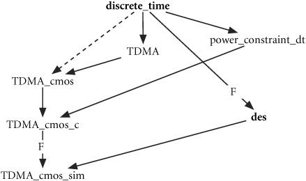
The first power-aware design study examines Rosetta’s capabilities for transforming and composing models to examine power trade-offs with respect to implementation technologies. The challenge is to determine whether it is best for a component from a TDMA receiver to be implemented in software, an FPGA, or an application-specific integrated circuit (ASIC) before prototyping the component. The approach chosen uses an activity-based power estimation model and simulation to determine activity in the component. The power model is specialized for each implementation technology using a refinement on a basic, abstract power model. The functional model is specialized similarly, changing the activity estimation based on the implementation technology. The power model and the functional model are composed using a product and a combinator applied to the result to generate a simulation model. The model can then be evaluated to determine the best implementation strategy. A graphical representation of this construction for FPGA, CMOS, and software implementations is shown in Figure 18.4.
The modeling process begins by determining the modeling goals. In the power-aware domain, the modeling process must support making trade-off decisions between implementation technologies. To achieve this, the relationship between the function being performed and how that function consumes power in each implementation technology must be understood. The specification anatomy must lead to a model that examines function and power consumption simultaneously.
To accomplish the trade-off analysis task, functional, power consumption, and power constraint models are required. The interaction between function and power consumption will give a system-level perspective on how power is consumed. The power constraint will indicate what limitations exist on available power. The interaction between power consumption, power constraints, and function will play a role in how the specifications are developed.
For the power-aware modeling activity, the basic Rosetta domain semi-lattice provides appropriate modeling domains for each model type. The power consumption model used is activity-based where power is consumed when a system changes state. The basic model makes no reference to any specific time representation, so the state_based domain is the most appropriate. The functional model is typically given as a discrete time model and best fits in the discrete_time domain. Finally, the power constraint is a simple constant value that cannot be exceeded. The fact that it is constant implies that the static domain is the most appropriate domain.
A discrete event simulation tool that can simulate state_based specifications is also assumed to exist. This is not a part of the standard Rosetta system, but could be provided by an external tool environment. The des domain in the semi-lattice defines requirements for the simulator, allowing functors and combinators to generate models for simulation. It is important to note that one could also explore these specifications using model checking, theorem proving, static analysis, or any number of formal and semi-formal techniques. This is simply a matter of defining a domain and functor for each technique, similar to the des domain.
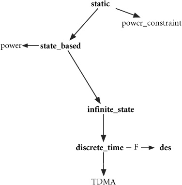
The relationships between domains in the semi-lattice and the connections between models and domains are depicted in Section 18.2. A segment of the domain semi-lattice is shown with the three models of the component’s function, an activity-based power consumption model, and a power constraint model. Also shown is the combinator that generates simulatable models.
The first modeling task is writing basic models for power constraints, power consumption, and device function. By keeping the models separate and in their own domains, each model remains focused and reasonably simple. Although some forethought must be given to how they will be composed, for practical purposes they can be written separately.
The power constraint (Figure 18.1) is constant across all time. Thus, the static domain is used to represent the static construct. The facet model simply defines a power variable and asserts that it must be less than the specified limit parameter. The power value is then exported to allow other models to reference it and assert constraints on it. By itself, the powerConstraint model does very little. Remember that it models the constraint on power consumption, not power consumption itself. It can easily be instantiated with a specific constraint. Without any other constraints on the exported power value, analysis tools cannot determine if the power constraint is or is not met.
When modeling power consumption using an activity-based model, power is consumed whenever the device changes state. Thus, the power consumption model (Figure 18.2) is defined in the state_based domain. By choosing the state_based domain rather than the more specific discrete_time domain, we define a common activity-based model that can be specialized for each individual model. The actual value used for state can be refined when the model is actually used. If a discrete_time model were used, the time value would need to be abstracted away if the model were applied in a domain without explicit representation of time.
Example 18.2. Power consumption model for the TDMA component.
facet powerConsumption(o::output top;
         leakage,switch::design real)::state_based is
 export power;
 power::real;
begin
 power' = power + leakage + if event(o)then switch else 0 end if;
end facet powerConsumption;
Unlike the power constraint model, the powerConsumption facet directly describes power consumption in a system. If an event occurs on the output, then the device is assumed to have changed state. In this situation, the device consumes power at a rate specified by the design parameter switch. If not, then only the power specified by leakage is consumed. Total power consumption is accumulated over time to determine the total device power consumption. This is a very naive power model, but it does reflect what is needed — a rough measure of how much power is consumed during the operation of the system.
Before moving forward, let’s examine what the product of powerConsumption and powerConstraint models means. The product is simple to specify:
limitedPower :: state_based is
 powerConsumption() * state_state_based.gamma(powerConstraint(5e-6))
 sharing {power};
The limitedPower model states that both powerConsumption and powerConstraint must be simultaneously satisfied. Alone, each model is satisfied by virtually any legal assignment. What is interesting in the composition is the role of the power variable. Because it is a visible part of both facet states, it is shared in the definitions. In other words, both models reference the same power item. Any value or property asserted on power must satisfy constraints from both facets. If either specification did not export the power item, this interaction would not occur.
In practical terms, the shared power variable means that if the power consumption model causes power to assume a value that is greater than 5e-6, then a contradiction occurs and the engineer knows a problem exists. All that is necessary now is to know when the device changes state.
The TDMA model is a discrete time model that defines functional requirements and takes into account delays through the circuit. Because the device is a time division multiplexer, it is necessary to include an explicit time value to capture the full functionality of the device. Thus, this model is defined in the discrete_time domain to allow this timing information.
The functional model (Figure 18.3) searches for a unique word in a bit stream and passes subsequent bits through until a specified number of bits has been seen. In effect, when the unique ID is detected, one packet of bits is passed through the TDMA receiver.
Example 18.3. Function model for the TDMA component.
facet TDMA(i::input real; o::output real; clk ::in bit
           uniqueID::design word(16);
           pktSize::design natural)::discrete_time is
  uniqueID :: word(16);
  hit :: boolean;
  bitCounter :: natural;
begin

  // Check to see if the unique ID has been seen and whether
  // a full packet has been transmitted.
  hit' =
    risingEdge(clk)
    and ((uniqueID = ID)or hit)
    and not (bitCounter >= pktSize);

  // If not transmitting bits, gather bits for unique ID
  uniqueID' =
   if risingEdge(clk)
      then if hit then x"0000"else sl(uniqueID,...)end if;
      else uniqueID
   end if;

  // If transmitting bits, update the bit counter.
  // Else set the bit counter to 0
  bitCounter' =
   if risingEdge(clk)
      then if hit then bitCounter+1 else 0 end if;
      else bitCounter
   end if;

  // If the unique ID has been seen, output the current bit.
  // Else continue to output the current bit.
  o' =
    if risingEdge(clk)
       then if hit and bitCounter =< pktSize then i else o end if;
       else o
   end if;

end facet TDMA;
The specification is not atypical of many discrete_time specifications. When the clock rises, the next state is calculated and the next output is generated. The first three specification blocks determine the next state by watching for a rising edge and then specifying values for variables hit, uniqueID, and bitCounter in the next state. The final specification block observes the state and determines what the next output should be.
Remember that our objective is determining how much power this particular device consumes over time to determine the best implementation choice. However, there is no mention of power or time anywhere in the functional model. This is exactly how it should be. The functional model should reflect the device’s function and should not be extended to include power and power constraints. That would defeat the entire purpose of Rosetta and domain-specific modeling. Timing information is present in the model and can be observed by analysis tools. However, using the abstract next function makes moving the model to different domains simpler. The functional model could be written in the state_based domain and moved to the discrete_time domain using a functor.
What will be done to understand the power consumption of this device is to compose the functional model and the power consumption model with the product operator:
TDMAPower(i:: input real; o:: output real)::state_based is
   TDMA(i,o,x"F0F0", 1064) * gamma(powerConsumption(i,o, 1e-9, 2e-8));
Like power in the previous product construction, i and o are shared by these models. When o changes based on some input to the TDMA device, the power consumption model will observe that change and will update its power value.
Actually constructing this model takes some additional work, but the basic idea of composing models begins to become more obvious here.
One key concept in the case study thus far is that each model is written using a different semantics, independently of other models. Although examples show how the models can be composed, thus far the models are independent and have no obvious connection other than names of parameters and variables. As shall be seen, the choice of names for items is critical when composing specifications.
The basic models involved in Figure 18.4 have been defined in the previous sections. The remainder of the figure involves defining transformations and compositions of models. Specifically, three things will be accomplished. First, the power constraints model will be refined to the state_based domain for composition with the power consumption model. Then the power consumption model will be specialized three times to reflect the different models of power consumption associated with CMOS, FPGA, and software implementations. Second, the functional model will be abstracted into the state_based domain, again to be composed with the various power consumption models. Finally, a combinator will be applied to create analyzable models from the specification products.
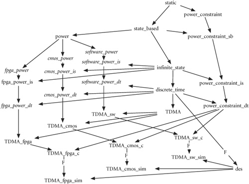
Figure 18.4. Full diagram, showing refinement and composition of device, power, and constraint models.
The naive approach to composing models is to simply construct a product directly without any model transformations. Unfortunately, this would eliminate all abstractions in our models and make analysis virtually impossible. Specifically, the common domain of these specifications is static, where no concept of time or state change is defined. The result would be a mass of equations that directly encode time and state change. This is not at all desirable.
The solution is choosing a domain where the desired analysis is best performed and constructing a model there. For this analysis, the state_based domain is selected, but other domains could be just as appropriate. The power consumption and power constraint models will be transformed so that they share this less abstract domain with the functional model (Figure 18.5). Although the functional model will lose the concept of time, the most important concept of state change vital to the activity-based power model remains. The specifics of time semantics are not needed.
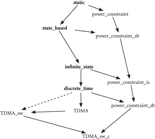
The process begins with the simplest activity — refining the power constraint model to include state. The refinement of the power constraint model that appears on the right side of Figure 18.4 is shown separately in Figure 18.6. Several functors are composed to construct the morphism that transforms the static power constraint model into a discrete_time model. This collection of transformations is actually quite trivial, as we simply assert that if a property is constant, it must hold at any time step.
In refining the power constraint model we are relying on a default interaction defined between the static and state_based domains. This interaction defines the functor static_state_based.gamma that transforms a specification from the static domain into a specification in the state_based domain. This functor and functors like it, i.e., that move down the domain semi-lattice, are simple to construct by simply constructing the extension that generates the more concrete domain from the more abstract domain. Whenever one domain is below another in the semi-lattice, the lower domain is created by extending the upper domain. In Chapter 15 these functors are given the name gamma and are defined between each pair of related domains.
In this case the functor used is defined in the interaction static_state_based and has the following signature:
gammaS[State::type]() from x::static to state_based(State);

gamma() from x::static to state_based;
There are two forms of this functor. Both assert that in the new specification, all terms from the old specification are true in every state. Thus, power must be less than the power limit in every state. The parameter in gammaS is used to provide a set of states to define the state type. In this case, a universally quantified parameter is used to allow the type to be inferred. If the state is held abstract, an identical functor, gamma, is available without the parameter. In this case, the state is unknown. Thus, gamma is initially chosen.
The functor can be used by including the following declaration in the specification:
powerConstraint_sb(x:: design real) :: state_based is
   static_state_based.gamma(powerConstraint(x));
A new facet now exists called powerConstraint_sb, parameterized over the power limit. This facet can now be used like any other. Of course, the declaration is not required. The functor may be used directly as a term anywhere in the specification where a facet of type state_based is expected.
With a state-based model of the power constraint constructed, the technology-specific power consumption models can now be constructed. To achieve this, the original power consumption model is transformed to represent power consumption in multiple different implementation technologies. The “refinement” performed here is achieved simply by instantiating parameters in the power consumption model with appropriate values. Of course, a more sophisticated transformation could be performed when more detail is known. However, an informed implementation decision can be made even in the presence of incomplete information using this model.
The technology-specific power consumption models are defined as follows:
CMOSpowerConsumption(i:: input real; o::output real) :: state_based
  is powerConsumption(i,o, 1e-9, 2e-8);

FPGApowerConsumption(i:: input real; o::output real) :: state_based
  is powerConsumption(i,o, 1e-9, 2e-8);

SWpowerConsumption(i:: input real; o:: output real) :: state_based
  is powerConsumption(i,o, 1e-9, 2e-8);
One does not typically look at parameter instantiation as refinement, but that is exactly what it is in this case. Instantiating the design parameters is literally the equivalent of substituting values for variables. Thus, the resulting specifications are in fact refinements of the original. Both the input and output parameters are retained to allow the facets to be composed structurally and combined with other specifications.
Now the new technology-specific power models can be composed with the power constraint. All exist in the state_based domain, so there is no need to transform specifications to other domains. The new facet models are easily defined as:
CMOSpowerLimited(i:: input real o:: output real) :: state_based;
  is CMOSpowerConsumption(i,o) * powerConstraint_sb(5e-6);

FPGApowerLimited(i:: input real o:: output real) :: state_based;
  is FPGApowerConsumption(i,o) * powerConstraint_sb(5e-6);

SWpowerLimited(i:: input real o:: output real) :: state_based
  is SWpowerConsumption(i,o) * powerConstraint_sb(5e-6);
These specifications all share a similar form and construct a product of a technology-specific power consumption model and a power constraint. Because the power constraint and the power consumption model export the power item, this value is considered shared between the specifications, and any constraints on it must be mutually consistent. This is precisely what is desired — a power consumption model limited by a specified power constraint. When we drive the values of i and o, the power consumption model will increase consumed power and the constraint model will compare with its constraint value.
What remains now is composition with the functional model. There are two equally valid approaches. The first refines the state_based power consumption models into the discrete_time domain and constructs a product with the functional model. The second abstracts the functional model to the state_based domain and constructs the product there. Both approaches are examined in the following sections.
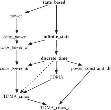
The refinement of constrained power consumption models into the discrete_ time domain is shown in Figure 18.7. The figure shows one of three constructions that generate the FPGA, CMOS, and software power consumption models on the left side of Figure 18.4. The approach mimics the approach used to move the power constraint into the state_based domain. Specifically, a functor is applied to the constrained power models that moves them from state_based to discrete_time.
In this case, the functor is actually the composition of two functors for moving from state_based to infinite_state and infinite_state to discrete_time. Defining the new functor is simply defining a function whose domain and range are facet types. Specifically:
gammaSBDT(f::state_based)::discrete_time is
  state_based_infinite_state.gamma.infinite_state_discrete_time.gamma
Functors in the built-in interaction libraries accomplish the refinement between individual domains. Getting the power models to the discrete_time domain is now a matter of applying the new functor:
let gammaSBDT(f::state_based)::discrete_time be
  state_based_infinite_state.gamma.infinite_state_discrete_time.gamma
  in
    CMOSpowerLimit_dt(i::input real; o::output real) :: discrete_time is
      gammaSBDT(CMOSpowerLimit(i,o));

    FPGApowerLimit_dt(i::input real; o::output real) :: discrete_time is
      gammaSBDT(FPGApowerLimit(i,o));

    SWpowerLimit_dt(i::input real; o::output real) :: discrete_time is
      gammaSBDT(SWpowerLimit(i,o));
end let;
The product can now be directly formed with the functional model and a discrete_time specification that accounts for power consumption results:
CMOS_TDMA(i::input real; o::output real) :: discrete_time is
   CMOSpowerLimit_dt(i,o) *
   TDMA(i,o,x"F0F0",1064);
FPGA_TDMA(i::input real; o::output real) :: discrete_time is
   FPGApowerLimit_dt(i::input real; o:output real) *
   TDMA(i,o,x"F0F0",1064);
SW_TDMA(i::input real; o::output real) :: discrete_time is
   SWpowerLimit_dt(i::input real; o:output real) *
   TDMA(i,o,x"F0F0",1064);
The alternative is moving the functional model to state_based and performing the composition there. The advantage is that the resulting model is simpler and more abstract. What we want here is the opposite of refinement — abstraction of the discrete_time model to the state_based domain. This is done using the alpha functors defined in the state_based_infinite_state and infinite_state_discrete_time interactions. Specifically, the alpha instance needed here is:
alphaDTSB(f::discrete_time)::state_based is
  (state_based_infinite_state.alpha.infinite_state_discrete_time.alpha)
Unfortunately, applying this instance of alpha may not always result in a successful abstraction. In addition to defining next concretely, the discrete_time domain defines time concretely as natural value. Thus, it is quite legal to have the following term in a discrete_time facet:
v@(t+5) = v+1;
Here, the time value is referenced directly rather than indirectly using next. Making its type abstract may cause problems if the addition operator is not defined on that abstract type. All is not lost. Remember that the state_based domain can be parameterized over the state type, making it possible to specify a state type that does have an addition operator. However, this does not truly result in an abstraction, but simply moving a complete definition to a new frame of reference.
Looking back at the functional definition, the time value, t, is never directly observed in the specification. Only the next function is used to specify movement from state to state. In this case it is possible to simply replace the discrete_time domain with the state_based domain. Thus, the functor from the built-in interactions can safely perform this operation.
With the abstract functional model in the state_based domain along with the power consumption model, the product can be formed in the state_based domain or a combinator can be used to generate a new model. This process is identical to that used when the power consumption models are made concrete, and thus will not be repeated here. The point of emphasis here is that if abstractions like this are to be used, care must be taken when writing specifications. When the intent is to abstract a model to a new domain, writing the model using vocabulary from the abstract domain has advantages. If this cannot be done, then writing a new alpha specifically for the situation is the most appropriate approach.
Following the transformation of the constraint models into the discrete_time domain where the functional model exists, products are used to construct a systems model. The functional model is used to generate activity information for the FPGA, CMOS, and software power consumption models while the power constraint model simply asserts a condition that must hold continuously in each model.
In both cases, an algebra combinator is used to construct a composite model from the product models. Details of the combinator are specific to the tool set used for performing the analysis. However, the interaction necessary for the composition and transformation has the form:
interaction discrete_time_des() between discrete_time and des is
begin
   begin translators;
   end translators;
   begin functors
      alpha() from des to discrete_time;
      gamma() from discrete_time to des;
   end functors;
   begin combinators
      alphaC() from x::des and y::des to discrete_time is
        alpha(x) * alpha(y);
      gammaC() from x::discrete_time and y::discrete_time to des is
        gamma(x) * gamma(y);
   end combinators;
end interaction discrete_time_des;
The necessary algebra combinator’s signature is is defined in the combinators section and has the signature:
gammaC(f::discrete_time,g::discrete_time)::des;
The final analysis models are:
CMOSsim(i:: input real; o:: output real)::des is
 gammaC(CMOSpowerLimit_dt(i,o), TDMA(i,o,x"F0F0", 1064));

FPGAsim(i:: input real; o:: output real)::des is
 gammaC(FPGApowerLimit_dt(i,o), TDMA(i,o,x"F0F0", 1064));

SWsim(i:: input real; o:: output real)::des is
 gammaC(SWpowerLimit_dt(i,o), TDMA(i,o,x"F0F0", 1064));
Figure 18.8 shows the combinator applied to construct simulation models from the product models. Like functors, combinators move models from one domain to another. The distinction is that combinators operate on pairs of models to generate a single model. Where products and sums cannot model the effects of interactions between domains, combinators can, because they generate new models.
This power-aware design example is among the oldest Rosetta specifications and has been used as an analysis example through many language revisions and tool instances. The structure of the specification is classic Rosetta. A collection of models is defined and composed to support cross-domain analysis. Although tool-specific analysis results are not germane to this presentation, we can speak to many of the emergent issues and common analysis results.
Now that we have the models, what do we do with them? These models have been analyzed in one form or another in Matlab, a custom Java analysis environment, and in the specialized Raskell Rosetta analysis environment. Across the board, analysis results depend more on the quality of data provided to models written, than on the tool or models used. However, we were able to learn things about interacting specifications in all tools that were beyond what simple simulation would show us.
Analysis results reveal that the software solution was the least power efficient. Our goal was demonstrating Rosetta modeling, not developing accurate power models, meaning the actual results should not be taken too seriously. However, we were able to observe changes in the power profile of the system with respect to changes in the execution profile. Ultimately this was our objective — understanding the impacts of local design decisions on global system-level properties. With more accurate models and a more realistic process, there is little question that analysis results would provide useful information.
In the most detailed analysis activity using Raskell, we were able to use an algebra combinator to move results from a functional analysis to the power analysis domain. This allowed us to estimate the power utilization based on the actual function being performed. The largest impact observed was in estimating the power cost of the software implementation. Because we were modeling software running on a CPU and the impacts of software state change on hardware state change, estimates were better than simply estimating power consumption on the CPU in general. However, this gain is not without cost. The actual models for power consumption are far more difficult to generate than are models for hardware implementations. This is a reflection of the intellectual distance between the software models and hardware realizations that actually consume power.
In addition to simulation analysis, formal techniques were used to perform some type analysis and some functional analysis. We used a theorem prover for these assessments. For power analysis, particularly using activity-based models, simulation is the best approach even though it is only semi-formal. Do not underestimate the value of formal semantics in simulation. Because the specification has a precise meaning, the correctness of simulation tools can be addressed. In this example, simulators were synthesized using formal techniques that guarantee their correctness. Such synthesis is not possible without Rosetta’s formal underpinnings.
Looking back at Figure 18.4, it should now be clear how the diagram is formed. Although morphisms in the diagram create some clutter, the shapes of different activities emerge, now that each activity has been identified. The original constraint models were refined as necessary to generate state_based or discrete_time models. These models were composed and models were generated using an algebra combinator. The resulting simulation models in the discrete event (des) domain were simulated and analyzed. Although Figure 18.4 is busy, it does represent the constructions necessary to construct the simulation models.
The models are presented as a complete system in Figures 18.9 through 18.11. The final power-aware case study model is split up between several packages for presentation. Figure 18.9 shows a package containing the several component models. Figure 18.10 uses the components package and defines power consumption models for each component. Finally, Figure 18.11 imports the packages containing component and power models, composing the models to define the final analysis models.
Example 18.9. Component models.
package powerAwareComponentModels() is
  export all;
  facet powerConstraint(limit::design real)::static is
    export power;
    power::real;
  begin
    power <= limit;
  end facet powerConstraint;

  facet powerConsumption(o::output top;
          leakage,switch::design real)::state_based is
    export power;
    power::real;
  begin
    power' = power + leakage + if event(o)then switch else 0 end if;
  end facet powerConsumption;

  facet TDMA(i::input real; o::output real; clk ::in bit
             uniqueID::design word(16);
           pktSize::design natural)::discrete_time is
    uniqueID :: word(16);
    hit :: boolean;
    bitCounter :: natural;
  begin

    hit' = risingEdge(clk)
      and ((uniqueID = ID) or hit)
      and not (bitCounter >= pktSize);

    uniqueID' = if risingEdge(clk)
           then if hit then x"0000" else sl(uniqueID,...)end if;
           else uniqueID
      end if;

    bitCounter' = if risingEdge(clk)
           then if hit then bitCounter+1 else 0 end if;
           else bitCounter
         end if;
    o' = if risingEdge(clk)
           then if hit and bitCounter =< pktSize then i else o end if;
           else o
         end if;
   end facet TDMA;
end package powerAwareComponentModels;
Example 18.10. Power consumption models.
use powerAwareComponentModels;
package powerAwarePowerModels()is
  export all;

  powerConstraint_sb(x::design real) :: state_based is
    static_state_based.gamma(powerConstraint(x));

  CMOSpowerConsumption(i::input real; o::output real) :: state_based
    is powerConsumption(i,o,1e-9,2e-8);

  FPGApowerConsumption(i::input real; o::output real) :: state_based
    is powerConsumption(i,o,1e-9,2e-8);

  SWpowerConsumption(i::input real; o::output real) :: state_based
    is powerConsumption(i,o,1e-9,2e-8);

  CMOSpowerLimited(i::input real; o::output real) :: state_based
    is COMSpowerConsumption(i,o) * powerConstraint_sb(5e-6);

  FPGApowerLimited(i::input real; o::output real) :: state_based
    is powerConsumption(i,o) * powerConstraint_sb(5e-6);

  SWpowerLimited(i::input real; o::output real) :: state_based
    is powerConsumption(i,o) * powerConstraint_sb(5e-6);

end package powerAwarePowerModels;
Example 18.11. Final model for the power-aware case study.
use powerAwareComponentModels;
use powerAwarePowerModels;
package powerAwareCaseStudy()is
  export all;

  sb2dt(f::state_based)::discrete_time is
    infinite_state_discrete_time.gamma.state_based_infinite_state.gamma;

  CMOSpowerLimit_dt(i::input real; o::output real) :: discrete_time is
    sb2dt(CMOSpowerLimit(i,o));

  FPGApowerLimit_dt(i::input real; o::output real) :: discrete_time is
    sb2dt(FPGApowerLimit(i,o));

  SWpowerLimit_dt(i::input real; o::output real) :: discrete_time is
    sb2dt(SWpowerLimit(i,o));

  CMOSsim(i::input real; o::output real)::des is
    gammaC(CMOSpowerLimit_dt(i,o),TDMA(i,o,x"F0F0",1064));

  FPGAsim(i::input real; o::output real)::des is
    gammaC(FPGApowerLimit_dt(i,o),TDMA(i,o,x"F0F0",1064));

  SWsim(i::input real; o::output real)::des is
    gammaC(SWpowerLimit_dt(i,o),TDMA(i,o,x"F0F0",1064));

end package powerAwareCaseStudy;