Chapter 4
Functional Analysis and System Design Models
In Chapter 3, we learned everything about requirements, including what system requirements are, how to write good requirements, where to obtain them, and how to manage them. Requirements define the system, but they cannot design the system. Requirements tell us what is desired for the system, but will not tell us how to make it happen. In other words, requirements are design independent; that is to say, the details to achieve those requirements are yet to be determined and there may be more than one way to fulfill those needs. Systems engineering uses requirements to drive the design in the right direction, but the use of a well-structured design process and a series of methods, models, and activities, leading to the final form of the system, bring it into being. System requirements need to be translated into technical specifications. This process of translation requires designers to have the necessary knowledge of the nature of the system and use appropriate models at the right time. When designing systems, especially complex ones, there are hundreds of thousands of factors and variables involved. It is nearly impossible to study the relationships of these factors to the design without using some kind of model. As the representation of the system, models are essential for designers to concentrate on the most critical factors of the design, simplifying the situation by ignoring the nonrelevant factors, and thus enabling them to provide a solution for the problem to be addressed. This chapter is intended to review the most commonly used models for system design once the requirements are developed; these models, although we call them systems engineering design models, are by no means solely developed for systems engineering. There are no such things as systems engineering models; systems engineering uses any models that are deemed useful for design purposes. As systems engineering is a relatively new discipline, it is an applied field; most of the models utilized in the field of systems engineering are borrowed from other fields, such as social studies, psychology, and operations research/simulation, to name a few. In this chapter, we will attempt to give a comprehensive review of some of the models that may be used in systems design; more specifically,
- Define models, review the benefits of using models and categorize models.
- Describe the functional modeling approach; define functions, how to derive functions, and introduce the functional flow block diagram (FFBD).
- Introduce function allocation model; introduce the processes that are involved in function allocation modeling.
- Review task analysis, cognitive task analysis, timeline analysis, link analysis, faulty tree analysis, failure mode and effects analysis, and statistical analysis models using experimental design.
It is worth mentioning here that the list of models reviewed in this chapter is far from complete; these are some typical models that most of the designs will utilize. There are some other models that we will cover in later chapters, as we do not want to make parts of the book redundant. There will be later chapters that are dedicated to specific models; for example, there will be a chapter solely on system simulation modeling. By exposing readers to these models, we are hoping that they will get a general idea of what kinds of models are available, what the inputs and outputs of these models are, and how these models can be applied to systems design.
4.1 What Is a Model?
In systems engineering, we study systems, trying to design a system based on needs, observing and measuring systems performance, and controlling system behavior. When studying a system, many believe that the best method is to use the system itself. It is beneficial if the nature of the system allows us to investigate it; it is direct and straightforward, but, unfortunately, studying the system itself is not possible most of the time. There are several reasons for this impossibility; firstly, the system may not yet exist. For a system design, especially a new one, most of the time we only have concepts; there is no real system available for us to manipulate. Secondly, sometimes it is not feasible to play with the system itself. Studying the system involves manipulation of and experimentation with the system variables; for example, changing the system layout, eliminating some factors or adding new components. These changes require inevitable interruptions to the current system and can be costly if the new design does not work the way we want it to. Moreover, sometimes it is even dangerous to experiment with the real system itself; for example, it may involve exposure to extreme environments, poisons, radiation, and so on. Under these circumstances, interacting with the real system is out of the question.
An alternative to studying the real system is to use a model of the system. A model is a representation of the real-world system; it is a duplication of the real system in a simplified and abstract form. A model may sound intriguing to most people, but, in fact, we use models and modeling techniques in our everyday life. For example, if we want to describe something, or tell a story, we need to use symbols, language, pictures, or numbers to let others develop a mental picture of the things we are describing or understand the story we are trying to tell. All the artifacts you are using, language, symbols, and pictures, are instances of models. Models are being used at every moment of our lives. Using models to describe the nature and interpret the causal relationships between different factors and variables has become a standard approach in every scientific and engineering discipline. With more technical data and high complexity involved in systems, models have become the inherent and critical part of designing, evaluating, documenting, and managing systems. It is hard to see any system being designed without using any type of models.
Using models in systems engineering can bring us many benefits. First, models allow us to study system concepts without directly interacting with the systems themselves. Some systems do not exist, except in their conceptual stages; some systems have a larger scope, beyond the capability of design teams, such as the social system and environmental systems, while other systems involve dangers that prohibit direct human interaction. Because models are duplicates of systems, they concentrate only on the most critical factors; ignoring the irrelevant factors enables us to focus on the most important aspects of system behavior. By doing this, we can make complex system relationships simpler and easier to be investigated. Second, it is much quicker to build a system model than to build the system itself, not to mention a lot cheaper too. Models range from simple sketches to scaled-down system mock-ups, and are a lot easier to develop, especially with modern technology and advanced computer hardware and software. During the process of system design, along with the evolvement of the system, many of the system parameters are not at the optimum operational level; constant testing, evaluation, and system modification are necessary, and the effect of system modification will not be identified until it is implemented. Interrupting the operating system without confidence in the model can cause lots of problems. Once the model is built and proven valid, that is, it truly represents the correct system behavior relationships, this enables designers to experiment and manipulate it with minimum effort, and various design ideas and modifications can be applied and tested without disrupting the real system, while maintaining a certain level of accuracy of prediction of the effects of the design changes on the system. In other words, even if our experiments fail or we mess things up here and there, we can start over again without costing much to the real system. Building systems models is one of the most important activities involved in systems engineering; it allows engineers to analyze the nature of the problems, leading to their solutions, thus achieving the technical goals of the design and bringing the greatest economic benefits.
4.1.1 Characteristics of Systems Models
The following is a list of the fundamental characteristics specifically of systems models:
- Systems models represent the system and its behavior in a valid, abstract, and effective way.
- Systems models use the minimum number of factors (variables) to describe the nature and characteristics of the system; these factors are considered most critical for the nature of the system and other factors can be ignored without affecting the validity of the model. In this way, we can simplify the problem so that it is solvable.
- Systems models describe the relationships between the factors, and system behaviors, effectively and accurately.
4.2 Model Categorization
4.2.1 Classification Based on Model Format
From the format of the model representation, models can be classified as physical, analogue, schematic, or mathematical models.
4.2.1.1 Physical Models
Physical models are the geometric duplicate of the system, usually in a scaled-down format; they concentrate on the physical, dimensional aspects of the system, including the geometric shape, orientation, color, and size; for example, a three-dimensional mock-up for a product prototype, a ground simulator for an aircraft cockpit system, or a layout plan for a plant facility. Physical models are used primarily for demonstration purposes and sometimes for experimenting with the system. For example, a building mock-up is utilized as a template for the layout of the departments, personnel, and machinery for a better flow. The most important aspects in a physical model are its physical dimensions and the spatial relationships between the components, such as the size and orientation of these components and the physical interaction between them.
4.2.1.2 Analogue Models
Analogue models, as the name implies, describe the relations between the system components. Unlike physical models, where there has to be a proportional duplication of the physical dimensions, in analogue models, although these are still physical in nature, the geometric dimensions are of little importance, but rather the interrelationships among the components are emphasized. For example, electric circuits are utilized to represent a mechanical system or a biological system. In analogue systems, it is not surprising to see that dots are being used as symbols to represent some system components.
4.2.1.3 Schematic Models
A schematic model uses a chart or diagram to illustrate the dynamics or structure of the system; unlike physical or analogue models, schematic models may not look like the real system physically. By proper coding of the system elements, using the appropriate symbols and constructs, a schematic system is intended to illustrate the dynamics of current and future situations or hierarchical static structures in that system. A typical example of the schematic model is an instructional diagram for a basketball play, for a coach to illustrate the ideas of offense or defense. A hierarchical chart of an organization is another common example of the schematic model.
4.2.1.4 Mathematical Models
Mathematical models describe systems using mathematical concepts and language. Based on observed system behavior and data, mathematical models formulate the system into a set of assumptions, variables, formulas, equations, and algorithms to illustrate the relationships between system variables. For example, designers often use linear programming models to optimize system resources allocation; or, a set of differential equations are used to describe the dynamics of system control. Mathematical models are very powerful tools to study the underlying fundamental laws and theories behind system behavior. They reveal the basic cause–effect relationships of systems variables, so that systems can be measured, controlled, predicted, and optimized. They have been commonly used in systems engineering. Of all the mathematical concepts being used in systems, operations research is one of the most popular mathematical modeling tools. It is an applied mathematical field that aids designers to make better decisions, usually concerning complex problems. As a matter of fact, the majority of the models covered in this book belong to the discipline of operations research. Operations research originated in military efforts before World War II for the optimal deployment of forces and allocations of resources; its modeling techniques have since been extended to address different problems in a variety of industries.
In developing a mathematical model, a typical procedure involves the following steps; first, the objective of the problem is identified by understanding the background to the problem and collecting the necessary information about it; second, based on the objective of the problem, a set of assumptions or hypotheses are developed to simplify the situation and prioritize the relevant factors. Assumptions make it possible for a system to be modeled mathematically and quantitatively. This is a critical step, as the validity of the assumptions will impact the validity of the model directly; a valid set of assumptions not only makes a mathematical model possible, but also captures the most critical and essential aspects of system behavior so that the model can reliably predict it. Third, based on the objectives and assumptions made, the most appropriate mathematical tools are chosen to develop the models. We are entering a wide field of applied mathematics; many tools are available for us to use to solve different problems, including algebra, probability and statistics, geometry, graph and network theory, queuing theory, game theory, and mathematical programming, to name a few. Mathematicians have prepared a rich field for us to explore. A good designer should be educated in advanced mathematical tools, so that the most appropriate tool will be selected for the right problem. Fourth, it is important to note that solving the model takes great effort. It is difficult to obtain an analytically definite solution for many complex models; for the purpose of system design, an approximate answer or near-optimum solution is often sufficient. Many techniques, such as graphical approach, numeric analysis, and simulation are very useful for reaching an empirical answer. Computer technology plays a vital role in solving models, making the solution process much more efficient. Last but not least, the results are implemented back into the system. Implementing the results requires another set of critical thinking skills, as many assumptions are made within the models; sometimes, we will find that the solutions are too ideal for real system implementation. For a feasible application, additional analysis is needed for practical purposes, such as sensitivity analysis and error analysis.
4.2.2 Classification Based on the Nature of the Variables
Based on the nature of the variables in the model, systems models can be classified as deterministic or stochastic models.
4.2.2.1 Deterministic Models
A deterministic model describes the relationships between deterministic variables; in other words, there is no randomness involved in the state of the models. Not only are the variables not random, the relationships are also fixed. With the same conditions, a deterministic model is always expected to produce the same results. Deterministic models can be complex in nature, and although there are definite answers that explain model behavior, such behavior is sometimes hard to obtain. For example, in control systems, some deterministic models are represented as differential equations, and it is difficult to express the state of the system explicitly at a particular point in time. Numeric analysis is one of the most popular approaches to approximate the answers in such a system. We can find many examples of deterministic models in our daily life; for example, most of the models in statics belong to this category, such as Newton’s three laws of motion. One particular type of deterministic model that needs our special attention is the chaotic model. This model is considered determinist because, theoretically, if the initial conditions are completely known for a dynamic system, its future state can be predicted exactly according to deterministic relations governed by a set of differential equations. But, in reality, it is impossible that the initial conditions of a system are known to the degree of precision required; thus, it is impossible to predict the future trajectory (behavior) of a chaotic system. That is why a chaotic system displays traces of random-like behavior.
4.2.2.2 Stochastic Models
In contrast to deterministic variables, there are random variables, which take a possible value from a sample space without certainty. Models that address random variables are called stochastic models, sometimes also referred to as stochastic processes. Probability and statistics are the most commonly used mathematical tools for developing and solving stochastic models. Randomness and uncertainty is everywhere in our daily life, as also seen in system design. Risks caused by environmental uncertainty can have a significant impact on system design efficiency and effectiveness. Understanding, analyzing, and controlling the level of randomness in the system design is very critical for system success. This implies that stochastic processes are widely applied throughout the system life cycle. Stochastic models take random input and produce random output. They use large samples to overcome individual indeterminacy, giving a likelihood of an outcome rather than a definite answer for given input values. In systems engineering, discrete stochastic models are very useful for analyzing system behavior and assessing design risks; these models include time series models, as seen in forecasting models, queuing models for a production process, and human factors performance data and modeling. We will be discussing each of these models in later chapters.
4.2.3 Other Types of System Model Classification
There are many other classifications of systems models, depending on the different perspectives of looking at them. For example, based on the scope of the models, there are macromodels and micromodels. Macromodels address issues in a large population and across a wide range of areas; for example, macroeconomics models to investigate financial situations in a region or a country. Micromodels, on the other hand, are usually focused on a small scope or problems in a single area; for example, models for a factory or for a production line are models at a microlevel, as these are very narrow and focused on a small area.
Based on the functions of models, systems models can be further classified as forecast models, decision models, inventory models, queuing models, economic planning models, production planning models, sales models, and so forth. These models are usually very specific, and we will also introduce these models in later chapters.
Model categories help us to understand the different formats, functions, and scope of the models, which, in turn, helps designers to choose the right models to solve problems. These model categories are not mutually exclusive; they overlap a great deal. For example, a mathematical decision-making model can be stochastic in nature and micro in scope. No matter what kind of model is being developed, there are some common features or things that need our attention across all different models:
- Models need to have a satisfactory level of validity. Validity refers to the level of closeness of the model to the real-world objects. The closer the model, the higher validity it has. Model validity reflects the accuracy and precision of the models; it depends on different factors, including the prior assumptions of the model and the variable selection/logic involved in the model. A valid model is believed to contain the most important and critical variables for the problem; thus, it is safe to use the model to replace the real-world objects for analysis and prediction of system behavior.
- Simplicity is preferred over complexity. When constructing models, given that the validity requirements are satisfied, simple models are desired for system analysis. Simple and clear models are easier to understand and quicker to build. If a simple model is sufficient to address the problem, there is no need to seek more complex models. In developing models, we should always start with simple methods, avoiding the use of intriguing mathematical concepts; remember that this is an applied field, so generalization is of little use. We should avoid developing models with no possibility of solving them. As a general rule, more variables are always believed to be more accurate than fewer variables, but we have to be careful about variable selection, and it is not always the case that the more the better; a balance between the complexity and numbers of variables should be sought to maintain a certain level of precision yet ensure a simple and clear model format.
In the following sections, a number of models that are used in system design and analysis are reviewed in sufficient detail. These models are most commonly found in almost all kinds of contemporary complex system design and systems engineering activities. We hope that, from the review, readers can acquire a comprehensive understanding of how these models can be applied in various stages of system design, what input and output factors are involved, and what special attention should be given when applying these models.
4.3 System Design Models
As mentioned before, systems engineering design is a process that translates intuitive user needs into a technically and economically sound system. This process involves many creative and critical thinking skills; we cannot develop a complex system based solely on recommendations, guidelines, and standards. Rigorous models are necessary for a precise transformation from the user’s needs to technical specifications. During the systems design process, almost all the different types of models can be found to have an application at certain stages. As a matter of fact, proper applications of modeling are essential for the success of the system design.
Before we get into the details of models, there are some common characteristics about system design models that need to be elaborated for readers to better understand them and their application within system design.
- System design models and methods address applied research questions. Basic research addresses fundamental research questions; these questions are basic in nature and often lead to general ground theories. These theories may be generalized to a wide range of fields. For example, the study of human skill performance is basic research; the theory behind such performance can be used to explain many kinds of human skill acquisition, such as learning musical instruments or learning how to fly an aircraft. Applied research, on the other hand, addresses specific research questions; for example, how does the location and size of the control button affect the user performance for a specific product interface? Applied research does not care as much about the generalization of the findings from the model; its focus is only on the specific product it is studying. The scopes of the applied research results are narrow and usually cannot be applied to other types of product for this reason. Systems engineering models only serve one specific system; their validity remains within the scope of the system. Although the finding may also make sense for other systems, there is no external validation guarantee for other types of systems unless the results are validated in those systems. Since basic research is conducted in ideal, well-controlled laboratory conditions, its findings have general meaning and wide applicability. Systems engineering models are usually conducted in actual design fields, with high internal but low external validity.
- Systems engineering models focus on prediction more than description. Scientific research is concerned more about describing the relationships between factors in nature. This is even more so for basic scientific research, as its purpose is to discover truths from evaluating nature around us; in other words, its purpose is the description of natural phenomena to try to give a scientific explanation for them. Systems engineering models, on the other hand, focus more on the prediction of behavior of systems and their components. For system design, most of the time when models are applied, the system is just a concept; the physical system does not yet exist. The purpose of modeling is to predict the future performance of the system, given certain inputs from the design and current system conceptual configurations. According to Chapanis (1996), application of models in systems development is much more difficult than that in basic research; since, in basic research, as the purpose of modeling is to discover and describe, even if a mistake is made, others can always carry out follow-up procedures based on the previous findings, with better data and analysis, to overcome the deficiencies in the previous studies; thus, the mistakes will be eventually corrected, because science is “self correcting.” In systems development, however, it is often not possible that many chances are given to create a design. Once a severe mistake is made, fixing it will significantly impact the system design efficiencies, causing delays and unexpected costs, sometimes even causing unrecoverable system failure. The accuracy of prediction is of utmost importance in systems development. When predicting system performance, applied systems models also rely on the findings from scientific theories; in other words, we cannot totally separate the prediction from the description. As mentioned in Chapter 2, engineering originates from science; designing a man-made system requires resources from Mother Nature—a good engineering model is always based on the solid foundation of scientific discoveries. Knowledge of both is a must for a good system designer. We should keep this mind; proper integration between basic scientific models and engineering design models is the key to the success of system design.
- System engineering models are not unique. Systems engineering is a relatively new field; all the models used in system design are borrowed and modified from other fields. This is due to the multidisciplinary nature of systems engineering. None of the models applied in systems engineering are unique; they were developed in other scientific or engineering fields, and have been adapted for systems engineering design purposes. For example, task analysis has long been used in psychology and social sciences to understand human behaviors; now it is used widely in systems engineering, especially to understand the interaction requirements between users and systems. In using the models, system designers should keep an open mind and be flexible. Since practical and specific answers are the concern, we should make effective use of all models appropriately in the design process.
- Systems models are used iteratively throughout the design process; during the process, it is not uncommon that one particular model is applied multiple times in different stages. For example, functional modeling is first applied after the requirements are completed to design the system-level functional structure. This is the typical usage of functional modeling at the conceptual design stage. In subsequent stages, functional models are also used to design the subsystem-level functional structures, with similar procedures but different starting points and levels of detail. This analysis is conducted iteratively until the final system functional structure is completed. Sometimes, results from the previous models are revisited or reexamined for verification purposes. For this reason, it is difficult to say that a particular model is only used in certain stages; it is very possible that a model will be used at every design stage, depending on the type of system being designed. By the same token, it is also possible that some models are not used at all for one system but used extensively in another system design. Similarly, designers need to keep an open mind when selecting appropriate models for the right system at the right time, by tailoring specific models to the system design needs.
- Systems models in design follow a sequence. Applications of certain models in systems design depend on the completion of other models, as some models take the results from others as input. This implies that certain models need to follow a particular series sequence. For example, functional modeling has to wait until requirement analysis is complete and task analysis is usually conducted after functional modeling is complete, as tasks are designed to serve certain functions. Understanding the prerequisite requirements for each model helps us to correctly construct the model at the right time with the correct input, thus increasing the efficiency of the system design.
In the following sections, commonly used systems design models are reviewed; please note that this is not an exhaustive list of models for system design, as some models are covered in other chapters. The intention of this review is to illustrate how different models are applied in the systems engineering context, for readers to get some basic understanding about the benefits and limitations of using models in systems design.
4.3.1 Functional Models
Functional modeling and analysis is one of the most important analyses in systems design; its intention is to develop a functional structure for the system, based on the systems requirements. Regardless of what kind of system is being designed, ultimately it will provide functions to meet user needs. In other words, user needs are fulfilled through system functions. Functional modeling and analysis is the very next step after systems requirements analysis, to identify what system functions shall be provided, what structure shall these functions should follow, and how these functions shall interact together in an optimal manner to achieve users’ needs efficiently. Functional models provide a picture of what functions that system should perform, not how these functions are implemented. In model-based systems engineering (MBSE) design, we want to evolve the system from one model to another, following a strictly defined methodology and a tightly controlled process, to minimize unnecessary changes and rework. This top-down approach will ensure a natural transition between models; going beyond the model’s scope and over-specifying the details before its maturity often cause rework issues. It is a common mistake that, in system functional models, physical models are blended within the function, leading to partial understanding or even an incomplete picture of the functional structure, narrowing the potential problem-solving space for future models.
4.3.1.1 What Is a Function?
Functional models address system functions. What is a system function? As defined in Chapter 2, a system function is a meaningful action or activity that the system will perform to achieve certain objectives or obtain the desired outputs to support the overall system mission or goals. The common syntax for defining a function is as follows:
Verb + nouns + (at, from, to …) context information
A system function has the following characteristics:
- A function is an activity or an action that the system performs, driven by the system requirements and regulated by technology and feasibility; a function is a desired system behavior. Including a verb is usually a typical way to identify a function; for example, “deposit check” or “withdraw cash from checking account” are two functions for an ATM system, while “user friendly” is definitely not a function, since there is no active verb in the phrase. It may define a property of a function, but not a function itself.
- A function can be performed at different levels; in other words, functions are hierarchical within the system architecture. A function may be accomplished by one or more system elements, including hardware, software, facilities, personnel, procedural data, or any combinations of these above elements. A higher-level function is accomplished by a series of lower-level functions; that is to say, higher-level functions are decomposed by lower-level functions.
- Functions are unique; there are no redundant functions unless redundancy is one of the functions to be achieved. For example, in enhancing system reliabilities, redundant functions are often provided, to be activated when the original function fails. Other than for this reason, functions should be unique, as space and resources are limited in system design.
- Functions interact with each other. From the same level of functional structure, each function takes inputs from the outputs of other functions, while providing outputs to yet other functions. All the functions work together cohesively to support the overall system’s highest-level function: the system mission.
System functions are derived based on the requirements; to develop an accurate functional model, designers need to understand the systems requirements, and, with help from the requirements analysis, to develop a functional behavior model that will effectively accomplish the system requirements. It is a translation process that turns users’ voices into a well-defined system functional structure. The development of system functions and their architecture relies heavily on designers’ knowledge, skills, and experiences with similar systems. Usually, a good starting point for functional modeling is scenarios and use cases, as these describe all the possible uses of the system, and all the functions are embedded within one or more scenarios if the scenarios are complete. An intuitive way for deriving the functions, especially for a new system, is to highlight all the verbs in the scenarios, and formalize and organize these verb phrases into a functional format. There is no standard method for functional development, as every system is different and everyone has different preferences for how to approach the system. As a rule of thumb, one should always start with the highest level of functions, the major function modules for the system mission, from the very top level (Level 0); the lower-level functions are specified for each of the major function modules. Through this decomposition process, perhaps with much iteration within each level, the complete functional model can be developed.
4.3.1.1.1 Input
Functional modeling uses information from system requirements analysis, including scenarios, use cases, analysis of similar systems, and feasibility analysis.
As mentioned earlier, taking this input information, designers start to identify the highest level of functions and decompose the higher-level functions into lower-level functions through an iterative method. Functions are formally defined, including the desired technical performance measures (TPMs) for the functions, such as power, velocity, torque, response time, reliability, usability, and so on; function structures are developed and traceability between functions and requirements, and between functions, is recorded.
4.3.1.1.2 Results
The output of the system functional modeling is development of a complete list of (1) systems functions and their hierarchical structure and (2) the interrelationships between system functions at different hierarchical levels, represented by the functional flow block diagram, or FFBD. The FFBD describes the order and sequence of the system functions, their relationships, and the input/output structures necessary to achieve the system requirements.
4.3.1.2 Functional Flow Block Diagram (FFBD)
A functional flow block diagram (FFBD) is a multilevel graphical model of the systems functional operational structure to illustrate the sequential relationships of functions. An FFBD shall possess the following characteristics:
- Functional block: In the FFBD, functions are presented in a single rectangular box, usually enclosed by a solid line, which implies a finalized function; if a function is tentative or questionable at the time the FFBD is constructed, a dotted-line enclosed box should be used. One block only is used to represent one single function, with the function title (verb + noun) placed in the center of the box. When one function is decomposed to a new sequence of lower-level functions, the new sequence should start with the origin of the new sublevel FFBD by using a reference block. A reference-functional block will indicate the number and name of that function. Theoretically, each FFBD should have a starting reference block. In Chapter 2 we presented an example of an FFBD; Figure 4.1 illustrates another example of a functional block diagram.
- Function numbering: An FFBD should have a consistent numbering scheme to represent its hierarchical structure. The highest level of systems functions should be Level 0 (zero); functions in the highest level of the FFBD should be numbered as 1.0, 2.0, 3.0, and so on. Note that the level number (0) is placed after the sequence number only for the highest level. The next level down after Level 0 is the first level of the FFBD; functions at this level should be numbered as 1.1, 1.2, 2.1, 2.2, 3.1, 3.2, 3.3, and so on. It can easily be seen that the numbers at this level only contain one dot, but are different from Level 0 as they have no zero in the numbering. The numbers easily inform us of the hierarchical relationships between functions at different levels; 1.1 and 1.2 are subfunctions of Function 1.0, while 3.1, 3.2, and 3.3 are subfunctions of Function 3.0. Using the same convention, functions at level 1 can be decomposed one step further to Level 2, with two dots in the numbering. For example, Function 1.2 can be further expanded to sublevel functions, 1.2.1, 1.2.2, 1.2.3, and so on if necessary. From this numbering system, it is easy to visualize the hierarchical relationships between different functions; we can immediately identify that 2.2.3 is a sublevel decomposition function of 2.2, and 2.2 is a child function of 2.0. Another benefit of using such a numbering system is to help designers gradually derive the system function structure step by step, in a very organized way, and avoid putting different levels of functions into the same level of the FFBD. Putting different levels of functions into one diagram is called recursive; it is a common mistake often found in FFBD development. Using the numbering system, it is easy to identify this error. Many software packages can detect the recursive error once the numbering system is in place.
- Functional connection: In an FFBD, functions are connected by lines between them. A line connecting between two functions implies that there is a functional flow between these two functions; that is, one function takes the output of another function as its input, either material, power, or information. If there is only a time-lapse between two functions and no other relationships, there should be no lines connecting the functions.
- Functional flow directions: Usually, for any function, a typical flow (go path) always goes in to its left-hand side (input flow) and goes out from its right-hand side (output flow). The reverse flow (from right to left) is used for feedback and checking flows. The top and bottom sides of the function are reserved for no-go flow; that is, the flow when the function fails. The flow exits from the bottom of the function and enters the diagnosis and maintenance functions (no-go paths). In the FFBD, no-go paths are labeled to separate them from go paths. Usually the flows are directional and straightforward; the directions form the structural relationships for the functions, such as series structures, parallel structures, loops (iteration loops, while-do loops, or do-until loops), and AND/OR summing gates. These constructs, together with their functions, define the functional behavior model for the system.
- Numbering changes: An FFBD is an iterative process; it is inevitable that deletion and addition of functions will occur during this process. With the deletion of existing functions, it is simple just to remove the function from the FFBD; for the addition of a new function, a new number needs to be assigned to the new item on the chart. The rule of thumb is to minimize the impact to the rest of the FFBD; although the new function might be placed in the middle of the FFBD, we do not need to renumber the functions to show its position, but we just choose the first unused number at the same level of the FFBD for the new function. In that way, the rest of the functions are not impacted (Blanchard and Fabrycky, 2006).
- Stopping criteria: The development of FFBD follows a top-down approach, as previously mentioned; it starts at the highest level of the functions and then, from there, decomposes each of the highest-level functions to its next sublevel, and so forth. It is imperative to have a stopping criterion for this decomposition process, because without it, decomposition can literally go on forever. While there is no well-established standard for such a criterion, it usually depends on the nature of the system and level of effort of the design. According to INCOSE (2012), a commonly used rule is to continue the decomposition process until all the functional requirements are addressed and realizable in hardware, software, manual operations, or combinations of these. In some other cases, decomposition efforts will continue until the FFBD goes beyond what is necessary or until the budget for the activity has been exhausted or overspent. In terms of the design tasks, however, pushing the decomposition to greater levels of detail can always help to reduce the risks, as this will lay out more requirements for the suppliers at the lower levels, making the selection of the components a little easier. We will revisit this process later in the functional allocation model.

The FFBD-based functional model is the backbone of the type A specification, which we discussed in Chapter 2. It defines the functional baseline and system behavior model, which serves as the first bridge between user requirements and technical system specifications. The success of the FFBD will lead to the final success of the system design.
We will use an ATM example from Chapter 2 to illustrate the FFBD structure. The following list shows the functions for a simple ATM system.
1.0 Verify account
2.0 Deposit funds
2.1 Deposit cash
2.2 Deposit check
3.0 Withdraw funds
3.1 Withdraw cash from checking account
3.2 Withdraw cash from saving account
4.0 Check balance
4.1 Check checking account balance
4.2 Check saving account balance
5.0 Transfer funds
The traceability of these functions is illustrated in Figure 4.2.

Hierarchical structure of ATM function model using CORE 9.0. (With permission from Vitech Corporation.)
An FFBD for simple systems can be developed simply by using paper and pencil, as the development process is very straightforward. However, for large, complex systems, the FFBD can easily become large and deep in the number of levels, and the interrelationships within the FFBD can become very complex. In this case, a computer-aided tool is desirable to manage such a large FFBD. Many systems engineering management software packages provide a capability for conducting FFBD analysis. As a matter of fact, the FFBD is a standard procedure for all kinds of systems design. In the next section, we will use Vitech’s CORE to illustrate how functional modeling is conducted.
In CORE, functional modeling is also called functional architectural modeling. Its purpose is to define system behavior in terms of functions and their structure, and to define the context in which functions are performed and control mechanisms activate and deactivate the system. Some of the basic functional model-related elements include
- Use case: In CORE, use cases are “precursors to the development of system scenarios”; they are extremely useful for gaining insights into the system’s intended uses, and thus help to lead us to the integrated system behavior models. As mentioned earlier, use cases and scenarios in the requirement analysis stages tell the stories of how the system will be used once built; they are one of the primary sources for extracting the functions. In CORE, a use case is defined by use case elements; as in UML, each use case involves one or more actors, defined by components in CORE; each use case is elaborated either by a function element, a programActivity element, or a testActivity element, depending on where the use case affects the system behavior (system design, program management, or verification/validation). A use case can be extended to other use cases. For example, for the ATM example, a use case could be “withdraw funds from the checking account”; the component would be “users” and would be elaborated by the “withdraw” function.
- Functions: In CORE, functions are actions that the system performs, just like the functions we defined in systems engineering; they are transformations that accept one or more inputs and transform them into outputs, providing inputs to other functions. A function is based on some requirements, it elaborates some use cases, and it is performed by one or more system components (hardware, software, or human). In the ATM system, “verify account,” “deposit funds,” “withdraw funds,” and “check balance” are all system-level functions.
- Item: In CORE, items are the resources or constraints necessary for functions to be performed, representing the flows for the functions. These resources include the materials, power, information, and user input. Items can be input to a function, output from a function or simply trigger a function to start. For example, a typical item for the ATM system’s “verify account” function is the passcode for the account; without the user input of this information, “verify account” cannot succeed.
- DomainSet: In CORE, DomainSet defines the conditions for the FFBD flow logic, such as defining the number of iterations or replications in a control structure, including the while-do, do-until, and IF-THEN conditions for the function decision logics.
- State/Mode: A state/mode in CORE represents certain states or phases in system operations. Recent development of MBSE requires integration with standard design methodology, such as SysML, which has been developed based on UML. System requirements specify different states/modes into which the system may evolve, which can be exhibited by systems components. States/modes are optional for system functional modeling if such items as phase structures are not necessary for the design.
Figure 4.3 illustrates the interrelationships between the elements in the system functional model, extending Figure 3.7.
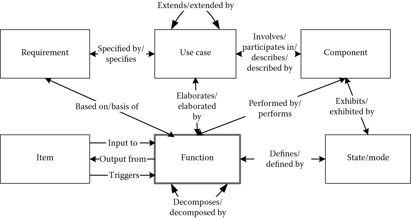
Defining functions in CORE is very straightforward, just as we described in requirement definition; when defining a function, we should also follow the element-relation-attribute (ERA) format. Table 4.1 illustrates the basic attributes and relations for a function in CORE.
Function ERA Structure
|
Element |
Attribute |
Relations |
Target Elements |
|
Function |
Description |
Allocated to/performs |
Component |
|
Doc. PUID |
Based on/basis of |
Requirement |
|
|
Duration |
Decomposed by/decomposes |
Function (at a lower level) |
|
|
Number |
Decomposes/decomposed by |
Function (at a higher level) |
|
|
Defines/defined by |
State/mode |
||
|
Inputs/input to |
Item |
||
|
Outputs/output from |
Item |
||
|
Triggered by/triggers |
Item |
Within CORE, the basic constructs for FFBD include
- Sequential construct: This is the most commonly used construct; it connects two or more functions together based on their input/output relationships. See Figure 4.4.
- Iteration: in CORE, iteration is used for a repeated sequence; it is similar to a while-do loop, as the iteration condition is tested at the beginning. For example, in the ATM system, if the user inputs the wrong passcode, he/she has two more attempts to enter the correct code; after three unsuccessful attempts, the system will lock the card and disable any further function. The condition (fewer than three unsuccessful attempts) is defined using DomainSet. See Figure 4.5.
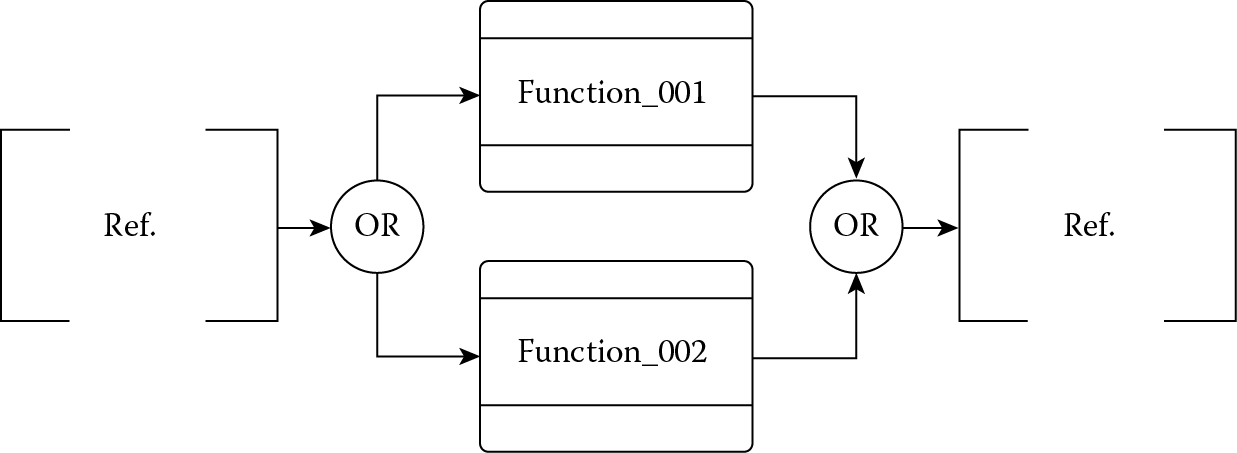
- Select (OR) construct: A select OR construct defines an exclusive OR path; only one path is enabled at a time. See Figure 4.6.
- Parallel (AND) construct: An AND construct defines a parallel path, where all the branches must be enabled at the same time. See Figure 4.7.
- Loop construct: This is similar to a do-until structure in computer program languages; it will repeat until a predefined condition is met. Unlike the iteration construct, the loop construct tests the condition after each iteration. Every loop is associated with a loop exit construct to allow exit from the loop. See Figure 4.8.
- Replicate construct: The replicate construct is the structure shorthand notation for identical processes that operate in parallel. The coordinates between these functions are defined in DomainSet in the coordinate branch. The replicate construct can be replaced by the parallel construct plus the coordinate branches. See Figure 4.9. A typical example of the replicate situation is a manager overseeing multiple checkout lanes in a grocery store.
When developing a FFBD, it is common to have different kinds of construct together within one diagram to elaborate the complex functional structure. For example, the FFBD in Figure 4.1 illustrates the high-level functional model for the ATM system.


The rest of the FFBD can be developed using similar methods until the lowest level of the FFBD has been reached. In developing the FFBD, although it is very straightforward and sometimes even intuitive, this also implies that there are no hard and fast rules to follow about how to conduct FFBD analysis; designers’ experiences and subjective judgment play a significant role in this process. There is a high degree of subjectivity in functional modeling, and there is no easy solution for this. Group decision making, more research findings about the system to be designed, and multiple rounds of iteration through verification and feedback are, perhaps, the only way to overcome this subjectivity. As is easily seen from the outcome of the FFBD and functional modeling, the system at this stage is still general in nature; that is, we only know what needs to be provided by the system, not how to achieve the functions. There is nothing said about the implementation of the system functions. Implementations of how functions are achieved need a further analysis, that is to say, allocating functions to systems components, which will be reviewed in the next section.
4.3.2 Functional Allocation
In Chapter 2, we briefly introduced function allocation methods and the functional allocation baseline developed from the allocation. Functional modeling produces a detailed structural and operational definition of the system functions, that is, what functions need to be performed and how these functions are structured to achieve the system mission. To implement these functions, systems elements are needed to carry out these functions; we need to know who is doing what functions. The typical system elements can be categorized into three basic forms:
- Hardware/physical elements: These are the tangible/physical components for building the system, whether static or dynamic, such as the facility, the system frame, parts, wires, and so forth. The allocation outputs are the quantitative and qualitative physical configurations of the hardware component.
- Software elements: These include the computer code and programs that are executed to control the system’s physical components. Software elements are responsible for the information flow and data management of system operations. The allocation output is the software configuration for the component, including the input/output specification and performance specifications, also including certain software platforms and interface structures.
- Human elements: These include the system operators/users and maintainers. These are the people that directly interact with the system and fix it if something goes wrong. The allocation outputs of the system functions to the human elements are the human staffing model (number of people and their scheduling), the operation and maintenance procedure, human system interaction specification and the skills and training requirements for the human elements.
Functional allocation starts with the results from the functional analysis, the function lists, and the FFBD, and just like functional modeling, there is no well-defined template or standard procedure to follow to produce a good allocation; knowledge of the system, familiarity with cutting-edge technology, experience with systems engineering, start-of-the-art design performance capability of hardware and software, and understanding of human capabilities and limitations, plus designers’ critical thinking skills and flexibility, are all possible inputs for conducting an allocation analysis. There is no guarantee that the first attempt will lead to a successful allocation baseline; like any other systems engineering analysis, allocation analysis is an iterative process, going through many rounds of iteration, and only from users’ feedback, verification and validation from simulations, and analysis and prototype testing may the most feasible allocation baseline be achieved.
Although there is no template for function allocation analysis, there are some general guidelines that can be followed. The transition from an FFBD-based functional model to a function allocation model always starts with a detailed FFBD analysis at the lowest level and function resource analysis for the lowest-level functions.
4.3.2.1 Resource Requirements for Functions
When all the functions are identified, we need to determine how these functions are accomplished. This is achieved by looking at the resources for each of the functions—that is to say: What are the inputs and outputs for the function? What are the controls/constraints for activating the function? And what types of mechanism are involved in the function? Example control/constraints include technical, social, political, and environmental factors; examples of mechanisms include human, materials, computer, facility, and utility support and so on. This process is performed for every function to determine the best way of achieving it. A graphical structure for this process is presented in Figure 4.10.

Identification of resource requirements for function. (Redrawn from Blanchard, B. S. and Fabrycky, W. J. Systems Engineering and Analysis , 4th edn. Upper Saddle River, NJ: Prentice Hall, 2006.)
Through this process, every function’s detailed resource requirements, as well as the quantitative technical performance measures (TPMs), can be determined. Based on the requirements, designers can seek the most feasible components (hardware, software, human, or a combination of these) to accomplish this function.
4.3.2.2 Allocation of TPMs
In performing the allocation procedure, a mixed process of top-down and bottom-up approaches is usually applied. First, the requirements and TPMs are allocated to the lower-level functions. This is generally a top-down process, and depending on the nature of the system structure, TPMs are allocated accordingly. For some quantitative measures, such as system reliability (usually measured by the failure rate or the mean time between failures [MTBF]), the allocation will be more vigorous, since the relationship between the components structure (e.g., series or parallel) and system reliability is well defined mathematically (the detailed models for reliability and related concepts will be described in Chapter 5). For many other TPMs, the allocation process is not that obvious; there will be a high degree of subjectivity involved. For example, to determine the human factors and usability issues in the lower levels, there are no equations for us to follow; the allocation is largely dependent on the personal experiences and capabilities of the person performing it and his/her understanding of the system and components. There is no shortcut for such an allocation other than iteratively reviewing and improving the design with teamwork and user involvement.
For most of the allocation, it is nearly impossible to achieve an optimal solution; with such a large degree of uncertainty and high level of complexity, it is not easy to formulate the problem into a well-structured optimization problem and provide a solution for it. Most of the time, we are seeking the most feasible solution within our understanding of the system functions, knowing the feasibility of current and emerging technology, and with help from the suppliers’ catalogue and global supply chain management resources. It is an iterative process that involves intensive decision making, trade-offs, prototyping, design, synthesis, and evaluation activities. It is believed that with this evolving design cycle, a feasible allocation baseline can be gradually achieved.
The product for the allocation analysis is the identification of the various system elements in terms of hardware components, software components, and human components, together with the data/information and TPMs associated with each element, or type B specification (the allocation baseline). The eventual goal of the function allocation is to know who/which is doing what function, how they are accomplished and by how much (the TPMs), providing a basic configuration for the system elements, so that system construction may be carried out in the next step.
Once the lowest level of system components and elements are identified and TPMs are allocated to those elements, the next step is to realize these components by configuring the assemblies for the system. When trying to work out the system components configurations, there are some limitations to be considered; one of them is that of the physical dimensions. There are certain requirements regulating the size and number of components to fit in a limited space. Layout and packaging design are issues that need to be considered in configuring the system structure, as mentioned in Chapter 2. Further development is needed to specify the assembly selection (Type C specification: product baseline), manufacturing process/procedures for these assemblies (Type D specification: process baseline), and materials specifications for the assemblies (Type E specification: material baseline). In developing these baselines, traceability has to be ensured to make sure the baselines conform with the systems requirements and design constraints.
In responding to these elements needs, designers need to conduct trade studies to select the most feasible alternative for realizing these components. Based on the functional allocation results, starting with the lowest level of the element architecture, elements providing similar functionalities are investigated together, and based on the current technology and manufacturing capabilities and the suppliers’ catalogue, possible elements with similar functionality are grouped together as the potential assembly of the system. This process, together with the trade studies results, evaluation, and testing, are carried out iteratively, until a feasible assembly plan is obtained (Type C: product baseline). Figure 4.11 illustrates this development process.

With the current globalization and supply chain environment, it is not always economically efficient to manufacture everything ourselves in-house; as a matter of fact, there are multiple suppliers that can provide similar components, and commercial off-the-shelf (COTS) items are the most cost-effective solutions for most of the system components selections. As mentioned in Chapter 2, when selecting a specific component fulfilling the function requirements, a series of trade studies and decision making is necessary to achieve the best feasible selection. Many of the decision-making models are conducted under uncertain situations and involve risks based on the predictions of future system performance. Decision making under risks and uncertainty are essential for systems design, as the design process constantly involves the optimization of limited resources. We will be covering the decision-making models in greater detail in Chapter 6.
As for the selection of the components, there are no standards for us to follow, as each system is different and involves different types of items but, generally speaking, there are some rule-of-thumb guidelines for the designer to follow; these guidelines have been practically proven to be efficient for saving costs and time. When selecting a component, we should follow the following order or sequence (Blanchard and Fabrycky 2006):
- Select a standard component that is commercially available. COTS items usually have multiple suppliers, and those suppliers are usually specialized and mature in terms of their manufacturing capabilities at an economically efficient stage of production. They are also certified and comply with quality standards, such as ISO standards, so we can take advantage of vast volume and high-quality items with the least cost involved. These suppliers often come with a high level of service for maintenance and repair of the components, which is another advantage when seeking more efficient and cost-effective system support.
- If such a COTS item is not available, the next logical step is to try to modify an existing COTS item to meet our own expectations. Simple modifications such as rewiring, installing new cables, adding new software modules, and so on, enable a function to be accomplished with minimum effort, without investing a huge amount of money to develop a manufacturing facility within the organization.
- If modifying an existing COTS item is not possible, then the last option is to develop and manufacture a unique component. This is the most expensive alternative and should be avoided if possible. As the last resort, we should not attempt to do everything all by ourselves; with the existence of a globalized supply chain, outsourcing and contracting should be considered for such a development, to take advantage of differences in costs of resources worldwide, including materials and labor costs.
The decision made concerning the design elements is to be documented in the Type C specification (product baseline) and the Type D specification (process baseline) if a manufacturing or developing process is involved.
4.3.2.3 A CORE Example of Detailed Functional Analysis
In CORE, the functional allocation model starts with expansion of the FFBD model to an enhanced version (the eFFBD model), by incorporating the resources and constraints information into the functions. To develop the eFFBD, we start with the FFBD results, adding the necessary resource information by defining the input/output of the functions (items) and assigning the functions to components. Their relationships can be seen from Figure 4.12 (functional relationship charts).

eFFBD of ATM functional model using CORE 9.0. (With permission from Vitech Corporation.)
Figure 4.12 illustrates an example for an ATM system eFFBD with items included.
Table 4.2 gives the ERA definition of the items and components elements.
Item Element ERA Definition
|
Element |
Attribute |
Relations |
Target Elements |
|
Item |
Accuracy |
Decomposed by/decomposes |
Item |
|
Description |
|||
|
Doc. PUID |
Input to/inputs |
Function |
|
|
Number |
Output from/outputs |
Function |
|
|
Precision |
Triggers/triggered by |
Function |
|
|
Priority |
|||
|
Range |
|||
|
Size |
|||
|
Size unit |
|||
|
Type |
|||
|
Item |
Abbreviation |
Built from/built in |
Component (lower level) |
|
Description |
Built in/built from |
Component (higher level) |
|
|
Doc. PUID |
Performs/allocated to |
Function |
|
|
Purpose |
|||
|
Number |
|||
|
Type |
Similarly to the functional model, the functional allocation model in CORE is conducted iteratively and also follows a top-down approach. Based on the allocation of TPMs and functional decomposition, plus the assessment of feasible technology, the components are allocated level by level, starting first with the high-level components and following the path of functional decomposition; the lower levels of components are then derived. This process continues until the lowest level of assembly is achieved; that is to say, COTS items will be obtained for that assembly, which is the stopping rule for the decomposition.
For communication between system components with external elements outside of the system boundary, interface and link elements are used to define such relationships. An interface element identifies the external components with which the system communicates, and the details of the interface are captured in the link element definition; that is, what kind of data is involved, what kind of hardware connection, software subroutine, and so forth. The relationships between the interface, links, and components are listed in Table 4.3.
Interface and Link ERA Definition
|
Element |
Attribute |
Relations |
Target Elements |
|
Interface |
Description |
Joins/jointed to |
Components |
|
Doc. PUID |
Comprised of/comprises |
Link |
|
|
Number |
Specified by/specifies |
Requirement |
|
|
Link |
Capacity |
Decompose/decomposed by |
Link |
|
Delay |
Through |
||
|
Delay units |
Connects to/connected to |
Component |
|
|
Description |
Specified by/specifies |
Requirements |
|
|
Doc. PUID |
Transfers/transferred by |
Item |
|
|
Number |
|||
|
Protocol |
For more information on these elements, readers can refer to the system definition guide published by the Vitech Corporation, which is available for download from www.vitechcorp.com.
4.3.3 Task Analysis Model
In system engineering design, task analysis is commonly used, primarily for specifying human–system interaction requirements and system interface specifications. It is used to analyze the rationale and purpose of what users are doing with the intended system, and to try to work out, based on the functional objective in mind, what users are trying to achieve and how they achieve the functionality by doing which tasks.
Task analysis has been a popular tool for applied behavior science and software engineering since the 1980s; it gained popularity due to its ability to include humans in the loop and its straightforwardness and simplicity. System designers use this method to investigate the human components allocation, especially their skills and the staff model based on the task requirements. In conducting task analysis, it is often found that the concepts of “tasks” and “functions” are confused; some functional models are conducted using a task analysis, and vice versa. In the previous chapters, we have briefly discussed the difference between these two. Here, for readers to better understand the task analysis model, let us spend some time again to distinguish between these two terms.
A function, as we have stated many times previously, is an action for which a system is specifically fitted, used, or designed to accomplish a specific purpose. In other words, it is a system action; it is what the system should do or perform. It is usually a more abstract goal or objective—although it involves a verb—but not an overly detailed activity. A task, on the other hand, provides such detail. According to the Merriam-Webster dictionary, a task is “a usually assigned piece of work often to be finished within a certain time.” In the systems engineering context, a task is an activity, usually performed by a system component, including hardware, software, or humans, in a timely manner to accomplish a particular function. A task is performed for a purpose; that purpose is a system function. So, system functions come first, and tasks come second, to serve the functions and enable them to be accomplished. Examples of functions in the ATM system design would be the “deposit” function or the “withdraw” function, and the tasks for these functions would be “insert card,” “input passcode using keypad,” “select a menu option,” and so on.
Now we know the difference between functions and tasks, this, in turn, implies that task analysis usually comes after the completion of the functional model, since tasks are dependent on functions. Just as Chapanis (1996) has pointed out, models in systems engineering follow a sequential order, in the sense that certain models use outputs from other models as inputs. Task analysis models are based on functional model structures; the tasks derived are associated with certain system functions, while functions are the rationale for task activities.
With this difference in mind, let us look at the definition of a task analysis model. Task analysis is a procedural model to identify the required tasks and their hierarchical structure, and produce the ordered list for all the tasks at different hierarchical levels. Based on this, task analysis is also called hierarchical task analysis (HTA).
4.3.3.1 Input Requirements
Starting from the functional model, inputs for task analysis include the function list, architecture, and the FFBD, supplemented with the understanding of the function and technological requirements, research findings from the literature, observations from the users, and expertise and experiences from the subject matter experts (SME).
4.3.3.2 Procedure
Designers take a team approach by integrating the information together for task analysis. Designers usually start from the highest level of the FFBD for each of the functions; based on the input, output, and resources/constraints information, designers use their experience and knowledge of the system and its functions, listing all the required tasks, describing them, putting them in order, and decomposing them into subtasks if desired. This procedure goes on until all the tasks are identified and no further decomposition is needed.
4.3.3.3 Output Product
The major output of an HTA is an ordered list of the tasks that users will perform to achieve the system functions. Additional information is also gathered for the tasks, including
- Information requirements for each task
- Time information for each task, including the time available and time required
- User actions, activities, and operations
- Environmental conditions required to carry out the task
Here is a sample task analysis for the ATM verification function:
- Verify user account information
- Insert bank card in the card reading slot
1.1 If card read successfully, go to 2
1.2 If card read fails, take out the card, and repeat 1
- Enter PIN
- If accepted, go to 3
- If rejected, repeat 2 until user has tried three times
- Choose “cancel,” go to 4
- Choose account menu
- Go to “withdraw” function
- Go to “deposit” function
- Go to “inquiry” function
- Go to “transfer fund” function
- Take card
From the above example, one can easily obtain the communication and data requirements for each task, and there are models available for the prediction of the time-required information. For example, in software engineering and human computer interaction, techniques such as GOMS (goals, operations, methods, and selection rules) and KLM (keystroke level model) are widely used for prediction of time information for a procedural task. These models provide an intuitive way to estimate the time and workload requirements for certain computer-related tasks, but they are subject to severe limitations; one of them is that they are deterministic models that do not account for errors and individual differences in experience and skills. Any unpredictable factors could skew the results, so that in the real-world context, justification and allowance are necessary for the application of these models.
Recently, another variation of task analysis has increasingly been used in systems design, which is called cognitive task analysis (CTA). Cognitive task analysis is an extension of the traditional HTA, with more focus on human cognition. Traditional HTA concentrates primarily on the physical activities of humans; these activities have to be observable for them to be recorded. However, in complex system interaction, many of the activities, especially mental activities, are not easily observed. For tasks that involve many cognitive activities, a slightly different approach than the traditional one is necessary to capture the cognitive aspects. There are five common steps involved in a typical CTA analysis:
- Collect preliminary knowledge: Designers identify the preliminary knowledge that is related to the system, to become familiar with the knowledge domain. Usually, the research findings from the literature and consultation with SMEs are utilized for the elicitation of such knowledge.
- Identify knowledge representation: Using the preliminary knowledge collected, designers examine it and allocate the task hierarchical structure, based on the traditional HTA structure. Designers may use a variety of techniques such as concept maps, flow charts, and semantic nets to represent the knowledge for each of the tasks.
- Apply focused knowledge elicitation methods: Based on the different representations of knowledge, designers may now choose the appropriate techniques for knowledge elicitation. Multiple techniques are expected for a better articulation of the knowledge. Techniques include interviews, focus groups, and naturalistic decision-making modeling; these are the most commonly used methods, and most of the techniques are informal.
- Analyze and verify the data: On completion of the knowledge elicitation, the results are verified using a variety of evaluation techniques, including heuristic evaluations and walkthroughs by experts, or formal testing involving real users to demonstrate the validity of the knowledge requirements for each of the tasks.
- Format results for the system design documentation: The results of the CTA are translated into design specifications so that they will be implemented in the design. Cognitive requirements, skill levels, and users’ mental models of task-performing strategies are derived to be translated to design specifications, especially the human–system interface aspects, so that systems functions are accomplished in an efficient way.
HTA and CTA are utilized widely, due to the simplicity and intuitiveness of the methods involved. The procedures involved in tasks analysis are very straightforward; with minimum training effort, a person can perform this analysis with little difficulty. However, good benefits also come with great challenges. The nature of the task analysis model requires, first, that the tasks to be investigated are observable, or can at least be partially observed. CTA uses knowledge elicitation of such mental tasks; this knowledge is also based on the research results concerning the cognitive resources for observed mental activities. Researchers and designers use their expertise and understanding of the system functions to develop the task and decompose it into subtasks to support the functions. This, in turn, implies another challenge for task analysis, which is the high level of subjectivity. There are no well-developed templates or standards for task analysis; the quality of the analysis is solely dependent on the capabilities of the person who is conducting it. Moreover, with a different person, it is entirely possible that the task analysis results would be different, and both sets of results may work for the design. To overcome the personal bias and distortion caused by subjectivity, task analysis usually takes a team approach by having a group of people involved to achieve a consistent outcome from the team. More research findings, data quality, and iterative checking/balance also help. These will facilitate the task analysis results to be more compatible with users’ true behaviors. For these reasons, task analysis models are most commonly used for design purposes, and are not suitable for evaluation, as there is no standard for right or wrong results from the task analysis.
4.3.4 Timeline Analysis Model
The timeline analysis model follows naturally from task analysis; it provides the supplemental time-required information for the task analysis, so that time-related workloads for various tasks can be identified.
In timeline analysis, graphical charts are often used to provide a visualization tool to lay out the sequence for all the tasks, and based on the research findings of each model, the time information is plotted on the charts to illustrate the temporal relationships of the tasks performed. Timeline analysis is very similar to the Gantt chart model, which is used to present project activity schedules. Figure 4.13 illustrates a simple time line analysis for a withdraw function for an ATM system.

4.3.5 Link Analysis Based on Network and Graph Model
Link analysis is a model derived from network and graph theory; it is concerned with the physical arrangement of the items so that the efficiency of operations between the items is optimized. These items include workstations, instrument panels, machines, offices, or any work areas involved. Network and graph theory is an important area of operations research, and since the 1970s, the application of network and graph theory has bloomed due to the increasing demand for large, complex facilities and layout planning. A graph is represented by a set of vertices and edges (sometimes called nodes and arcs/lines). A network is a graph with numbers associated with each edge or arc; these numbers could be the distance, cost, reliability, importance, frequencies, or any related parameters. Network models can be used to solve a variety of problems, including the decision tree, shortest path, minimum/maximum flow, matching and assignment, traveling algorithm, location selection, and project scheduling, to name a few. In industrial engineering, optimization using networks and graphs is commonly found to be applied to facility layout design and planning. In this chapter, we will only select several fundamental models to get readers started on the familiarization of network optimization models. For more in-depth discussion of graph and network theory, one should refer to a more advanced text on this subject such as Evans and Minieka (1992) or Tompkins et al. (2003).
The application of graph and network theory in systems engineering is also referred to as the link analysis model, as it studies the linkage between different elements within the system. Link analysis enables designers to visualize the spatial relationships of systems elements and quantify the parameters involved for these relationships; thus, the overall effectiveness of the links can be optimized.
4.3.5.1 Input
The primary inputs required for a link analysis are data from the functional analysis, functional allocation, and task analysis, plus knowledge of existing and emerging technology, similar systems, and any data collected during the requirement analysis stages, including the observation, interviews, and surveys from users.
4.3.5.2 Procedure
Regardless of what specific network model is being used, a general approach for link analysis involves the following steps:
- Identify the objective of the link analysis. What is the purpose of conducting such an analysis? What is the measure of effectiveness and efficiency for this particular problem; that is, are we trying to find the best layout to minimize the total traveling distance among elements? Or, are we trying to put the system elements together in such a way that the total importance index between elements is maximized?
- List all the elements for the link analysis, including the personnel and items. Based on the relationships between all the elements and the objectives, quantify the links between the elements, including the distances, frequencies, cost, and so forth.
- Measure the priority/importance score for each of the links if necessary.
- Develop the from-to matrix for the vertices (for the elements) and the arcs, based on the values assigned.
- Apply the appropriate algorithms to place the elements in the layout until all the elements have been assigned.
- Evaluate the final layout by calculating the score for the measures of effectiveness. Implement the layout based on the results.
To illustrate the above procedure, we will give one example based on graph theory to explain how the algorithm works.
Example 4.1
Five stations are being put in a limited space; the frequencies between the stations and their corresponding importance (or weightings) are given in Figure 4.14.
The weighted-frequency matrix is derived by multiplying the frequency of the pair with its corresponding importance score (or weighting). For example, the weighted importance between Stations 1 and 2 is 10, which equals the frequency score between 1 and 2 (2) multiplied by the corresponding importance score (or weighting) for the link between 1 and 2 (5). Find a layout for the five stations that maximizes the total sum of the weighted frequencies for the chosen links.
The procedure for graph-based link analysis is described as in the following steps:
Step 1. From the weighted-frequency relationship matrix, rank the all the arcs/links in descending order, as shown in Table 4.4. From the list, select the station pair with the largest weighted-frequency score. Ties are broken arbitrarily. For this example, Stations 4 and 5 are chosen to be placed in the layout first as they have the largest score (16) (Figure 4.15).
Ranked Weighted-Frequency Score for All Links
Link
Score
4–5
16a
1–4
15
2–5
14
1–2
10
2–4
9
1–3
8
2–3
8
3–4
5
1–5
0
3–5
0
a Indicates the chosen station to enter the layout.
Step 2. Now we need to find the third station to enter the layout graph. The remaining stations are compared in terms of the sum of the scores with respect to the selected pair from Step 1. Select the station with the highest score, as seen in Table 4.5. For this example, Station 2 is selected as it has the highest sum of scores (23) with respect to Stations 4 and 5 (Figure 4.16).
Step 2 Calculation
Candidate Station
4
5
Sum
1
15
0
15
2
9
14
23a
3
5
0
0
a Indicates the chosen station to enter the layout.
Step 3. Now we need to find the fourth station to enter the layout graph. The approach is similar to Step 2, except now we have three stations already in the graph. This step involves assessing the sum of the scores of the remaining stations by comparing the sum of the scores when placing the station in one of the faces of the graph. A face of the graph is defined as a bounded region, enclosed by three or more station nodes. For this step, there is only face, 2–4–5. Table 4.6 lists the sum of scores for the two unassigned stations. Based on the comparison, Station 1 is chosen to be placed in the face of the graph (Figure 4.17).
Step 3 Calculation
Assigned Stations
2
4
5
Sum
1
10
15
0
25a
2
8
5
0
13
a Indicates the chosen station to enter the layout.
Step 4. Now we have only one unassigned station (3) left. The task now is to determine in which face to place Station 3. There are four faces available in total from the results of step 3: 1–2–4, 1–2–5, 1–4–5, and 2–4–5 (do not forget this face). The sum of the scores for putting Station 3 in the four different faces are compared, and we choose the placing which has the highest total. See Table 4.7 for the comparison (Figure 4.18).
Step 4 Results
Faces
Sum of Scores When Station 3 Is Placed in the Face
1–2–4
8 + 8 + 5 = 21a
1–2–5
8 + 8 + 0 = 16
1–4–5
8 + 5 + 0 = 13
2–4–5
8 + 5 + 0 = 13
Note: The total weighted frequency score is 23 + 25 + 21 = 69
a Indicates the chosen station to enter the layout.
The steps above give an algorithm to find the layout with the maximum score. If the object is to find the minimum score for any possible reason, the above steps would still be the same, except to change the rule to select the lowest score instead of the highest score. The procedure is straightforward and very similar to finding the highest score; as an exercise, readers can try to find the layout for a minimum-weighted score for the above example. We have also included some exercise questions at the end of the chapter for further practice.
In some cases, obtaining the final link structure is not sufficient; designers need to translate the link diagram to fit a limited area. Imagining that the stations are actually departments, if distances are not taken into consideration, how would we translate the final results into a rectangular floor plan? There are many procedures that have been developed to aid in this planning, such as Muller’s systematic layout planning (SLP) procedure (Tompkins et al. 2003). These procedures are quite straightforward and intuitive; they are not difficult to understand. Readers can refer to other texts for a more detailed explanation of those procedures. A same layout planning for the above example is illustrated in Figure 4.19.
4.3.6 Center of Gravity Model for Facility Location Planning
Project managers and system designers often face the decision of selecting a location for the system facility. There are several options when selecting a location; one can expand the existing facility if there is adequate space for it—this option is more desirable because it costs less than other alternatives. A second option is to add a new location. For example, it is economical to build a facility near a source of raw materials to cut down the cost, or to outsource the manufacturing process. This option has more impact than simply adding extra capacity, since it involves more investment and has more influence through interaction with the new environment and society. The decision shall be made based on the system mission and requirements, to bring in more benefits and save costs, with other constraining factors in mind, such as the political, legal, and financial conditions of the selected location.
There are many models for location planning; selection of the model depends on the different objectives and constraints in which the planning is involved. Here we introduce a model called the center of gravity method. It is widely used in operations management to find the location of a facility that minimizes total travel time or costs to various destinations.
The center of gravity method uses a map to show all the destination locations. Using an (x, y) coordinate system, each of the destination locations can be identified on the map, such as the one in Figure 4.20.
If the quantities to be shipped to every location are equal, then coordinates for the center can be easily determined by the following formula:
ˉx=∑xin
x¯=∑xin (4.1)ˉy=∑yin
y¯=∑yin (4.2)where:
(xi, yi) is the coordinate pair for the ith destination location
n is the total number of locations
So, for the above example represented by Figure 4.20, the center of gravity is located at
ˉx=∑xin=x1+x2+x3+x4+x5+x66=4+10+19+21+11+76=12
ˉy=∑yin=y1+y2+y3+y4+y5+y66=3+6+6+11+13+156=9
as shown in Figure 4.21.
If the frequency (or quantity) of the shipment to each location Qi is not equal, then a modified weighted average is used to determine the center of gravity.
ˉx=∑Qixi∑Qi (4.3)
ˉy=∑Qiyi∑Qi (4.4)
For the above example, suppose the daily shipment frequency and quantities per shipment are as shown in Table 4.8. The weighted-average-based center of gravity is
Frequency
Quantities per Shipment
Total Q
S1
1
600
600
S2
2
400
800
S3
2
450
900
S4
5
250
1250
S5
3
400
1200
S6
4
100
400
ˉx=∑Qixi∑Qi=4(600)+10(800)+19(900)+21(1250)+11(1200)+7(400)600+800+900+1250+1200+400 ≅13.54
ˉy=∑Qiyi∑Qi=3(600)+6(800)+6(900)+11(1250)+13(1200)+15(400)600+800+900+1250+1200+400≅9.19
Please note that the above example assumes a deterministic shipment amount. In the stochastic case, the shipment quantity is a random variable, and follows some distribution function. In this case, the expected value is used for the quantity. For example, for S1, the shipment has the discrete distribution shown in Table 4.9. The expected value for the shipment quantity for S1 is given by the following formula:
E(Q1)=∑4j=1P1jQ1j=(0.2)(250)+(0.3)(400)+(0.1)(600)+(0.4)(800)=550
The formulas for Equations 4.3 and 4.4 become
ˉx=∑E(Qi)xi∑E(Qi) (4.5)
ˉy=∑E(Qi)yi∑E(Qi) (4.6)
A comprehensive review for the probability and statistical models is given at the end of this book in Appendix I.
4.4 Summary
Models are the abstract representation of the real system; they play an important role in systems, as they make complex systems simpler, so that the relationships between critical variables may be investigated. In this chapter, we defined the models in the systems engineering context and identified the major characteristics and benefits of using models in systems design. Models used in systems design can be classified into different categories, based on different perspectives. Based on the format, models may be categorized as physical models, analogue models, schematic models, or mathematical models; based on the variable types, they may be categorized as deterministic or stochastic models; based on the model’s scope, there are macromodels and micromodels; based on the model’s functions, there are forecast models, decision models, queuing models, and so forth. For each of the categories, descriptions of their significance and examples were given for a better understanding.
In terms of systems engineering models, it is noted that most systems design models are applied research from nature and focus on the prediction of system behavior; they are borrowed from other disciplines and modified for systems design purposes. These systems engineering design models are used iteratively in the system life cycle, with various levels of detail for different iterations.
Systems models and analysis are the main theme for this whole book; in almost every chapter, different types of models are reviewed. In this chapter, some commonly used design models were discussed, while trying not to overlap too much with the remainder of the book. Two major design models, the functional analysis and function allocation models, were reviewed in great detail. System functions were defined, and their characteristics, syntax, and the FFBD graphical method was explained. As a hands-on exercise, we used CORE as a platform to illustrate how to use software to conduct FFBD analysis. An ATM system was used as the example of function analysis. Function allocation and the relationship between different design baselines (Types A, B, C, D, E) were discussed at the end of the FFBD analysis section. Following functional modeling, task analysis and cognitive task analysis (CTA) were introduced to obtain the interaction design specifications between the users and the system. The input and output for these models and general procedures are given for conducting a task analysis.
The last section of this chapter was dedicated to link analysis. The two most commonly used link analysis models were reviewed: graph-based layout planning and center of gravity models to determine facility location. The procedures were elaborated with numeric examples and their application to systems were discussed.
Problems
- Define a model. What are characteristics for a model?
- What are the benefits of models? What are the possible limitations of a model?
- List all the models categories based on format, variables, scope, and functions. Give one example of each.
- If you were a systems engineer, explain why you would want to use models in your design and what the unique characteristics of systems engineering models are compared to other disciplines, say psychological models?
- Define functions and describe the characteristics of systems functions.
- Develop the functional models (functions and their architectures) for the following elevator system scenario:
A passenger elevator is located in a four-story building in a College of Arts and Sciences Building. It has two doors on each floor, opening on two sides for passengers to access the elevator. The elevator operates on a 24/7 time basis, unless it fails, or there is an emergency, or it is time for a monthly maintenance check, performed by a certified technician.
- Download CORE from vitechcorp.com, and use CORE to develop an FFBD for Problem 6.
- From Problem 7, pick one function, conduct the resources management analysis for this function, and identify the input/output and constraints for this function. Define “item” for this information and develop an eFFBD using CORE.
- Based on your experiences and observations with elevators, develop an HTA to transport a passenger upstairs.
- What are the differences between task analysis and cognitive task analysis (CTA)?
- Describe how traceability is ensured between system design baselines (i.e., Type A to B to C, D, and E)?
- A manufacturing company produces one part for a major automobile customer in five locations throughout a country. Raw materials will be distributed to these five locations from a centralized warehouse within the country. The weekly quantities to be delivered to these five locations are assumed to be same. The following table shows the coordinates for the five locations. Use the center of gravity method to determine the coordinates for the location of the warehouse. Draw the five locations and the warehouse on graph paper.
Location
x
y
L1
2
3
L2
8
2
L3
7
7
L4
9
5
L5
4
13
- A grocery supplier is trying to determine the best location for its new distribution center within the area. The coordinates and daily shipping amount (in lbs) from the center to the six stores is listed in the following table. Determine the coordinates for this new center using the weighted-average center of gravity method
Location
x
y
Amount (lbs)
L1
2
2
100
L2
3
5
150
L3
5
4
125
L4
9
6
200
L5
7
8
200
L6
4
10
350
- A grocery supplier is trying to determine the location for its new distribution center within the area. The amounts shipped to the nearby six stores are random variables. The coordinates and daily shipping amount (in lbs) and probability distribution from the center to the six stores are listed in the following table. Determine the coordinates for this new center using the weighted-average center of gravity method.
Location
x
y
Amount (lbs) and Probabilities
L1
2
2
P(100) = 0.5, P(150) = 0.5
L2
3
5
P(50) = 0.1, P(100) = 0.5, P(150) = 0.4
L3
5
4
P(100) = 0.3, P(125) = 0.7
L4
9
6
P(200) = 1
L5
7
8
P(80) = 0.2, P(200) = 0.2,P(300) = 0.6
L6
4
10
P(100) = 0.3, P(200) = 0.3, P(350) = 0.4
- Shown below is a relationship matrix for five departments, conduct a graph-based link analysis to maximize the total adjacent importance score.

Rate
Score
V (very important)
8
I (important)
6
M (moderate)
3
U (unimportant)
1
- Consider the layout for a five-department design (sizes are ignored). The material flow is given in the following table.
A
B
C
D
E
A
—
25
0
6
20
B
—
5
15
30
C
—
20
0
D
—
10
E
—
- Develop the final adjacent graph using the graph-based link analysis procedure to maximize the total adjacent flow. What is the final total flow amount?
- Fit the layout of the five departments from (a) into a rectangular block.