
Chapter 6
Decision-Making Models in Systems Engineering
Humans make decisions every day. These decisions range from ones with longer-term impacts, such as whether to take a job after college or go to graduate school to everyday decisions such as what to eat for lunch. Similarly, in systems design, decisions are being made constantly on a daily basis. This is because
- The resources involved in systems design are always limited. One of the most important objectives and challenges for systems engineers is to utilize limited resources in the most effective and efficient way; this goal is achieved only through a well-thought-out decision-making process.
- The systems engineering design process is itself an iterative decision-making process. Systems engineers make decisions in a continuous basis; from the development of requirements, selection of design concepts, choice of appropriate components, and optimization of system parameters to the final system installation and operation, design decisions are being made at different levels. Due to the complex nature of the designs, these design decisions usually involve multiple criteria and, sometimes, high-risk stakes and uncertainties, which will have significant impact on the quality, cost, and safety of the designed system.
With a high degree of uncertainty, multiple criteria, and, sometimes, conflicting decision goals involved, systems engineers strive to find the best solution for these types of complex decision-making problems within a relatively short period of time. To simplify these problems, proper models are necessary to articulate and formulate the decisions. In this chapter, we will review some of the commonly used models for solving decision-making problems in the systems engineering context. These models are largely quantitative in nature, providing a rigorous foundation for systems engineers to address the decision-making problems at different levels. On completion of this chapter, readers should have a good understanding of the decision-making problems within the systems context in general, know how to identify decision objectives, criteria, and factors, formulate problems into solvable mathematical models, and obtain feasible solutions. More specifically, the following concepts and topics will be covered in this chapter:
- A rigorous definition of decision-making problems and the characteristics/elements of a decision-making problem
- Review of deterministic decision-making models
- Illustration of the difference between decision risks and uncertainty; review of decision-making models under risks and uncertainty
- Review of commonly used decision-making models including utility theory and decision tree models
- Review of the decision-making problems that involve multiple criteria; more specifically, ranking of the decision criteria by analytical hierarchical process (AHP) methods
At the end of the chapter, a brief summary is given to help readers to organize the concepts discussed in the text, providing a general framework for considering decision problems in complex systems design.
6.1 Elements of Decision Making
Decision-making is a high-level human cognitive process to select a preferred action among several alternatives; it is a process in which “a person must select one option from a number of alternatives” with “some amount of information available” and under the influence of context uncertainty (Wickens et al. 2003). Some of the unique elements of systems engineering decision-making tasks include the following:
- It has a goal to achieve. All decision-making tasks are carried out to achieve a specific goal. The goal is usually associated with a certain degree of optimization, that is, to maximize overall revenue or to minimize the cost of the completion of a project.
- It is a selection process. There is usually more than one approach to achieve the goal; these different approaches are called decision alternatives. Such alternatives are usually complementary to each other, that is to say, one alternative is better in one aspect but worse in another. If an alternative, A, is better in every single aspect than a second alternative, B, it is said that Alternative A dominates Alternative B; a dominating decision makes the problem easier to solve. In most cases, it is not always easy to obtain dominating alternatives. Given a set of candidate alternatives that are complementary, a decision maker’s job is to select the best alternative that serves the decision goals, usually by using some types of decision aids and models.
- Realistically, any decision-making tasks are subject to some time constraints; decision makers have a limited time window to make that decision. However, for most systems design decision-making problems, time is usually not an issue; system engineers should have sufficient time to put together all the information, develop decision models, and solve the problem. Any decisions regarding systems designs should not be rushed. So, for decision making in systems engineering, we usually assume that the decision time is not a factor, and there is no time limit to reach a decision. Decision making under time pressure is a slightly different problem and has been studied extensively in psychology and human factors; for example, Rasmussen’s skill, rule, knowledge (SRK) model of behavior and Klein’s recognition-primed decision (RPD) model. These models differ from the decision-making models in systems engineering in the sense that they are mainly qualitative and empirical in nature, involving many heuristics.
- Decision making usually involves uncertainty. Uncertainty can be characterized as the unknown probability or likelihood of a possible outcome of a decision or the lack of complete information on which to base a decision. Uncertainty plays a significant part in modeling the decision-making process in systems engineering and is usually modeled by the use of probability and statistics theories. Readers should be familiar with the fundamental concepts of probability and statistics to understand the concepts and models of this chapter. For a preliminary study and review, please refer to Appendix I of this book.
Regardless of the nature of the problem, the decision-making process usually consists of a sequence of six activities, described as follows:
- Identify the problem and outline the goals to be achieved. These goals serve as criteria against which to compare different alternatives for solving the problem.
- Gather the data that is necessary to solve the problem.
- Based on the data collected, generate alternatives to achieve the goals. An alternative is a candidate solution for the problem.
- Articulate the problem by using the appropriate model, integrating all the data and decision criteria together to evaluate the alternatives.
- Evaluate the alternatives using the model. Based on the decision criteria, the best alternative is selected.
- Consider practical implications and limitations and execute the decision actions.
In the following sections, we will introduce the most commonly used decision-making models in systems engineering, starting from the decision-making models under risks and uncertainty, followed by utility theory, the decision tree, and the decision-making models for multiple criteria, including the AHP model. Most of these models originate from the normative models based on probability and statistics, which can be found in most operations research texts.
6.2 Decision-Making Models under Risks and Uncertainty
To explicitly explain the procedure for solving decision-making problems, let us denote the following:
m: numbers of alternatives
n: numbers of possible future events that could happen
Ai: the ith alternative, where i = 1, 2, …, m
Fj: the jth future event, where j = 1, 2,…, n
Pj: the probability that the jth future event will occur in the future, where j = 1, 2, …, n
Eij: the payoff if the ith alternative is selected and jth future event occurs.
Based on the above notation, a decision-making problem can be formulated by using the decision evaluation matrix (see Figure 6.1).

Decision evaluation matrix. (Redrawn from Blanchard, B. S. and Fabrycky, W. J., Systems Engineering and Analysis , 4th edn, Prentice Hall, Upper Saddle River, NJ, 2006.)
For decisions under certainty—that is to say, the future event is certain, meaning that there is only one future possible and Ei is the payoff if the ith alternative is selected—the solution to the problem is very straightforward; that is to select the alternative that can maximize the payoff (in terms of the cost, Ei would be negative, so the maximization of the payoff would still apply), as shown in Equation 6.1:
(6.1)
6.2.1 Decision Making under Uncertainty
For decision making under uncertainty, it is assumed that all future events are possible and there is no information about the likelihood (probability) of the future. Five possible decision criteria can be used to make a decision: Laplace, maximax, maximin, Hurwicz, and minimax regret. To illustrate these criteria, let us consider the following example.
A company is considering building a retail store in a new location to increase sales revenue. The company can choose not to build the store, but to use other stores to fulfill demand, or build the store in three different sizes, small, medium, or large. There are three possible levels of future demand for this new location, which can be quantified as low demand, medium demand, and high demand. For different levels of demand, a certain alternative yields a unique payoff. For example, if a small store is built, and if the demand for the new market is small, an annual equivalent payoff value of $10,000 will be obtained. The annual equivalent payoff value for all the alternatives are presented in the decision evaluation matrix shown in Table 6.1 (in thousands of dollars).
Decision Evaluation Matrix for Store Size Example (in thousands of dollars)
|
Possible Future |
|||
|
Low Demand |
Medium Demand |
High Demand |
|
|
A 1 : Do nothing |
5 |
6 |
7 |
|
A 2 : Build small |
10 |
12 |
12 |
|
A 3 : Build medium |
7 |
15 |
15 |
|
A 4 : Build large |
− 3 |
5 |
20 |
Before we proceed to solve the problem by using different decision criteria, the first thing to do is to examine the alternatives, to see if any dominated alternative exists. If the payoff of Alternative A is superior (better) than that of Alternative B for all future events, then Alternative A dominates Alternative B, or Alternative B is dominated by Alternative A. Mathematically, a dominated alternative can be defined as follows:
An alternative Ai is dominated by an alternative Ai′ if for all possible future events, Fj, j = 1, 2, …, n, Eij ≤ Ei′j; and for some future Fj′, Eij′ ≤ Ei′j′.
A dominated alternative should be eliminated from the pool of alternatives. For the above example, it is easy to see that A1 (do nothing) is dominated by A2 (build small) or A3 (build large), so A1 should be eliminated from consideration. The problem thus can be simplified to Table 6.2. A further examination finds that there is no alternative in Table 6.2 that is dominated by other alternatives.
Modified Decision Evaluation Matrix for Store Size Example (in thousands of dollars)
|
Possible Future |
|||
|
Low Demand |
Medium Demand |
High Demand |
|
|
A 2 : Build small |
10 |
12 |
12 |
|
A 3 : Build medium |
7 |
15 |
15 |
|
A 4 : Build large |
− 3 |
5 |
20 |
6.2.1.1 Laplace Criterion
In the absence of the probability of future events, it is not possible to assume one event is more likely than another, but rather we assume that they are all equally possible. This assumption is based on the principle of insufficient reason (principle of indifference), or the Laplace principle, which states that if n possibilities are indistinguishable from each other except for their names, then each possibility should be assigned an equal probability of 1/n. As Laplace (1902) indicates,
The theory of chance consists in reducing all the events of the same kind to a certain number of cases equally possible, that is to say, to such as we may be equally undecided about in regard to their existence, and in determining the number of cases favorable to the event whose probability is sought. The ratio of this number to that of all the cases possible is the measure of this probability, which is thus simply a fraction whose numerator is the number of favorable cases and whose denominator is the number of all the cases possible.
Based on the Laplace principle, the probability of the occurrence of future events for the above example is 1/3. Or, in other words, the best alternative to be selected is the one that has the largest arithmetic average. This is illustrated in Table 6.3.
Laplace Criterion (in thousand dollars)
|
Low Demand |
Medium Demand |
High Demand |
Laplace Criterion |
|
|
A 2 : Build small |
10 |
12 |
12 |
(10 + 12 + 12) ÷ 3 = 11.33 |
|
A 3 : Build medium |
7 |
15 |
15 |
(7 + 15 + 15) ÷ 3 = 12.33 |
|
A 4 : Build large |
− 3 |
5 |
20 |
(− 3 + 5 + 20) ÷ 3 = 7.33 |
From the results, it is apparent that A3 (build medium) is the best choice.
6.2.1.2 Maximax Criterion
The maximax criterion selects the alternative with the largest payoff value out of the best payoff values for each alternative. For each alternative, determine the best payoff (or largest value); the maximax criterion chooses the alternative with the best of the best outcomes. For this reason, the maximax criterion is also called the “optimistic” criterion, as it only looks at the best-case scenario for each alternative. Mathematically, the maximax chooses the alternative Ai with the largest value of maxj Eij, or maxi{maxj Eij}. Considering the example Table 6.2 presents, the maximum payoff value for each alternative is shown in Table 6.4.
Payout according to the Maximax Criterion (in thousand dollars)
|
Alternative |
|
|
A 2 : Build small |
12 |
|
A 3 : Build medium |
15 |
|
A 4 : Build large |
20 |
From Table 6.3, the maximum number is 20; thus, the selection based on the maximax criterion is A4 (build a large store).
6.2.1.3 Maximin Criterion
Contrary to the optimistic maximax criterion, the maximin is the pessimistic criterion that selects the best of the worst-case scenarios for each of the alternatives. The maximin chooses the alternative Ai with the largest value of minj Eij, or maxi{minj Eij}. Consider the example Table 6.2 presents; the minimum payoff value (worst-case scenario) for each alternative is shown in Table 6.5.
Payout according to the Maximin Criterion (in thousand dollars)
|
Alternative |
|
|
A 2 : Build small |
10 |
|
A 3 : Build medium |
7 |
|
A 4 : Build large |
− 3 |
From Table 6.3, the maximum number is 10; thus, the selection based on the maximin criterion is A2 (build a small store).
6.2.1.4 Hurwicz Criterion
The maximax and maximin criteria above present the two extreme ends of decision making. But, realistically, a decision maker is usually neither extremely optimistic nor pessimistic. Most of the times, a decision maker compromises between the maximax and maximin criteria. The Hurwicz criterion adds certain levels of realism into the formula, by calculating the weighted average between the maximax and maximin using a coefficient of optimism, indicated by α, with 0 ≤ α ≤ 1. The Hurwicz criterion is represented by Equation 6.2:
(6.2)
So, a decision maker would select the alternative with the largest value of Hi, or maxi Hi. α is called the coefficient of optimism and 1 − α is the coefficient of pessimism. One can easily see that if α = 1, the Hurwicz criterion becomes a maximax criterion and if α = 0, then it becomes a pure maximin criterion. So we can say that the maximax and maximin criteria are two special cases for the Hurwicz criterion. The selection of α is largely subjective; it depends on the decision maker’s personal feelings regarding optimism and pessimism. A different α will change the results of the decision. As an example, using the matrix from Table 6.2 and an α of 0.8, the results are presented in Table 6.6. Clearly the choice would be A4, as it has the largest payoff value of $15,400.
Example of the Hurwicz Criterion with α = 0.8 (in thousand dollars)
|
|
|
Hurwicz with ? = 0.8 |
|
|
A 2 |
12 |
10 |
0.8(12) + (1 − 0.8)(10) = 11.6 |
|
A 3 |
15 |
7 |
0.8(15) + (1 − 0.8)(7) = 13.4 |
|
A 4 |
20 |
− 3 |
0.8(20) + (1 − 0.8)(− 3) = 15.4 |
6.2.1.5 Minimax Regret
The minimax regret criterion uses the concept of opportunity cost to arrive at a decision. An opportunity cost is also called a regret; a regret for an alternative for a certain future event is the difference between the payoff for that alternative and the best payoff for that future. For example, for the future event of low demand, the best payoff is $10,000 dollars, which is alternative A2, so the regret for A2 is 0, the regret for A3 is 3, which is the difference between the payoff for A3 (7) and the best payoff (10), and similarly, the regret for A4 is 13. The regrets for all the alternatives are listed in Table 6.7.
Regret Matrix
|
Low Demand |
Medium Demand |
High Demand |
Maximum Regret |
|
|
A 2 : Build small |
0 |
3 |
8 |
8 |
|
A 3 : Build medium |
3 |
0 |
5 |
5 |
|
A 4 : Build large |
13 |
10 |
0 |
13 |
The minimax regret criterion selects the alternative with the best of the “worst” regrets, or the minimum of the maximum regret. For the above example, the minimax criterion recommends alternative A3 (build medium).
The minimax criterion is similar to the maximin, as it also looks at the best of the worst-case scenarios. However, since the minimax criterion applies to the regret rather than to the payoff value itself, it is believed not to be as pessimistic as the maximin approach.
6.3 Decision Making under Risks
Risks, in the context of systems engineering, lie between the two extreme cases of certainty and uncertainty. With risks, future events are still random but we have knowledge of the explicit probability of the occurrence of future events; in other words, information about Pi, i = 1, 2, …, n is available for future Fi, i = 1, 2, ..., n, and .
The most commonly used criterion for decision making under risks is the expected value criterion. The expected value criterion chooses the alternative that yields the maximum expected payoff value. The expected value of an alternative is calculated as the sum of the products of the payoff value and its corresponding probability, or mathematically
(6.3)
For the example from Table 6.2, if we know that P1 = 0.25, P2 = 0.45, and P3 = 0.30, then the expected value for A2 is
The expected values for all the alternatives are presented in Table 6.8. Clearly, from Table 6.8, the expected value criterion suggests A3 would be the best choice.
Expected Value Criterion
|
Probability |
0.25 |
0.45 |
0.30 |
|
|
Demand |
Low |
Medium |
High |
Expected Value |
|
A 2 : Build small |
10 |
12 |
12 |
0.25(10) + 0.45(12) + 0.30(12) = 11.50 |
|
A 3 : Build medium |
7 |
15 |
15 |
0.25(7) + 0.45(15) + 0.30(15) = 13.0 |
|
A 4 : Build large |
− 3 |
5 |
20 |
0.25(− 3) + 0.45(5) + 0.30(20) = 7.50 |
Using the expected value for decision-making risks seems rational, as it selects the maximum expected payoff value. However, this criterion may not capture the true behavior of humans when making decisions under risks, as different people might have different preferences regarding the values of the risks. To illustrate, let us assume two lottery alternatives between which a decision maker must choose: Lottery 1 (L1): There is a 100% chance (certainty) of receiving $100; Lottery 2 (L2): There is a 50% chance of receiving $300 and a 50% chance of receiving nothing. Let us apply the expected value criterion to these two alternatives. Clearly, the expected values are EX(L1) = $100 and EX(L2) = 0.5(300) + 0.5(0) = $150. The expected value criterion recommends us to choose L2 over L1 as it has a larger expected value (150 > 100), but, in the real world, many people are not willing to risk a 50% chance of receiving nothing, but would rather play safe, walking away with a guaranteed $100. The decision is made based on people’s individual perceptions of the risk, and how much the risk is worth to each individual person; the perception of risks varies among different individuals, which cannot be interpreted accurately by the expected value. We introduce a more comprehensive model to address individual decision making under risks, the Von Neumann-Morgenstern Utility Theory, in Section 6.4.
6.4 Utility Theory
John Von Neumann and Oskar Morgenstern (1944) developed a model of expected utility (VNM utility) to replace the expected value criterion to represent individual preferences regarding risks. The utility, defined by Von Neumann and Morgenstern, is a quantitative measure of decision preferences of choices associated with risks. To define the utility functions, let us first revisit the decision problems involved with risks.
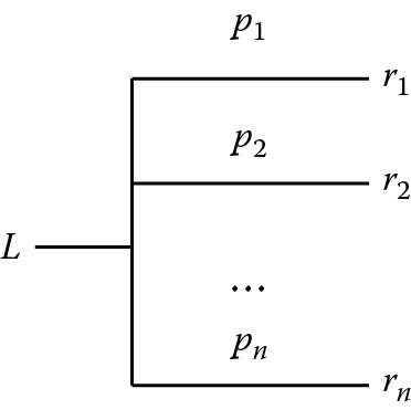
In VNM utility theory, a decision option is denoted as a lottery, as an analogy to gambling options. A lottery is a situation where an individual (or agent) will receive one reward ri with a probability of pi, (i = 1, 2, …, n), from n mutually exclusive outcomes. A lottery is denoted as L(p1, r1; p2, r2; …; pn, rn) and can be easily represented by a tree structure, with the tree branches representing the possible outcomes, as shown in Figure 6.2.
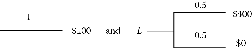
For the lottery examples mentioned above, in Lottery 1 (L1), one receives $100 with certainty:

And in Lottery 2 (L2), there is a 50% chance of receiving $300 and a 50% chance of receiving nothing:

In the above examples, as we have mentioned, although L2 has a higher expected value, in reality most people would choose L1 instead, simply because L2 involves risks while L1 has no risks at all. Utility theory is intended to incorporate the effects of risks in choosing between lotteries, assuming we only can choose one lottery, not both. If L1 is preferred over L2, we denote this choice as L1pL2; or we say that L1 has a higher utility than L2.
If we are allowed to change the probability for lottery L2—say we will increase the probability of receiving the $300 from 0.5 to 0.8—this results in a new lottery, L3.

With this increased probability, most people would now be willing to choose L3, if they believe L3 is indifferent from L1 as the risk becomes lower, then we say that L1 and L3 are equivalent, or L1iL3. This implies that L1 has the same utility as L3.
To address the effects of risks on lottery decision making, we use utility to replace the monetary value to reflect the decision makers’ feelings about the risks involved in lotteries. With the preference and indifference of lotteries defined, we can now give a formal definition of utility as follows (Winston 1994, 2005):
A utility of a reward ri, denoted as u(ri), is the value of the probability qi, that makes the following two lotteries equivalent:

The utility u(ri) can be thought as a number qi where a decision maker feels indifferent between receiving ri for certain and the risk qi between the most favorable and least favorable rewards. This utility is usually expected to be different between different decision makers; it is a subjective preference that an individual feels about the value of the risks with respect to the amount to be received. It is a common practice that makes the following assumptions about the most favorable and least favorable rewards:
ri is a reward value between the most favorable and least favorable rewards, u(ri) = qi, and 0 ≤ qi ≤ 1.
When comparing the lotteries, we use utility to replace the actual monetary reward to represent the decision maker’s preference concerning the combined effects of the monetary value and its associated risks. The utility function allows decision makers to tie their personal attitudes to the rewards and risks to alternatives (lotteries); thus, the decision made is more realistic and individual using the expected value criterion. Let us look at the following example to see how the utility function is derived and how we use it to choose between different lotteries. Consider three lotteries as follows:

If we apply the expected value criterion, we will find that all three lotteries have the same expected value. Readers can easily verify that all the lotteries have the same expected value of $5. So, under the expected value criterion, decision makers should feel indifferent between these lotteries. But, in reality, different decision makers will have different preferences concerning them. Let us see how the utility model can be applied to rank these three lotteries. For all three lotteries, it is easy to see that the most desirable reward is $20, and the least desirable outcome is −$5. For all other rewards (ri = $0, $5, $10), a decision maker is asked to determine the probability pi so that the decision maker feels indifferent between the two lotteries.

Suppose that, for $0, the decision maker is indifferent between

And for $5, the decision maker is indifferent between the following two lotteries:

and for ri = $10, the decision maker is indifferent between the following two lotteries:

Using the above definition of indifferent lotteries, the decision maker can transform the original lotteries L1, L2, and L3 to their equivalent lotteries , , and , shown in the following, such that they only contain the most favorable and the least favorable outcomes:

is called a compound lottery because it consists of multiple lotteries within . A compound lottery such as can be reduced to a simple lottery by combining the probabilities of the same reward. For example, for $20, the probability is 0.5(0.9) + 0.5(0.6) = 0.75, and for −$5, the combined probability is (0.5)(0.1) + (0.5)(0.4) = 0.25, so is reduced to the following simple format:

From the new lotteries , , and , since they all contain either the most desirable or least desirable outcomes, one can easily make a decision by comparing the probabilities of receiving the most desirable rewards; since 0.8 > 0.75 > 0.4, we can obtain the preferences for these three lotteries as . This implies that, for this decision maker, L1p L3p L2.
Another way to rank these three lotteries is to use the utility function. According to the definition of the utility, we have u($20) = 1 and u(−$5) = 0, and, by definition, we can obtain the utility values for other rewards since the decision maker is indifferent between

So, u($0) = 0.6. Similarly, we can obtain the utility function values for the remaining rewards: u($5) = 0.8 and u($10) = 0.9.
With all the utility function values known, we can calculate the expected utility for each of the lotteries, which will give the same ranking results. The expected utility can be defined as the following:
For a given lottery L:(p1, r1; p2, r2; …; pn, rn), the expected utility, written as E(U for L), is
(6.4)
Using expected utility, we can easily choose between two lotteries by the following criteria:
Thus, for our example above, we have
So, based on the expected utility criteria, we can rank these three lotteries as L1pL3pL2, since 0.8 > 0.75 > 0.4, which gives us the same results as using the composite lotteries.
To use expected utility theory, Von Neumann and Morgenstern proposed and proved the following four axioms as prerequisites.
Axiom 6.1: Complete Ordering Axiom
For any arbitrary two lotteries, L1 and L2, exactly one of the possible must be true: (1) L1pL2, (2) L1iL2,or (3) L2pL1.
Axiom 6.2: Transitivity Axiom
If L1pL2 and L2pL3, then L1pL3.
Axiom 6.3: Continuity Axiom
If L1pL2 and L2pL3, then there exists some value of p, 0 < p < 1, such that where

Axiom 6.4: Independence Axiom
The independent axiom implies that for the same decision-maker, two lotteries mixed with a third one will remain the same preference order as when the two lotteries are compared independently of the third lottery. Suppose that we L1pL2 and for any 0 < c < 1 and comparing with another lottery L3, the same preference will hold, that is,

These four axioms will define a rational decision maker; expected utility theory applies if and only if these four axioms hold true.
By defining the utility function, we can derive information about a decision maker’s attitude to risks; he/she is either a risk-seeking, risk-neutral, or risk-averse person. This information can be obtained by looking at the certainty equivalent (CE) and risk premium (RP) values.
A CE of a lottery L, denoted as CE(L), is the reward r such that the decision maker is indifferent between the lottery L and receiving a certain reward r. Then CE(L) = r. For example, if a decision maker feels indifferent about the following two lotteries
then CE(L) = $100.
Knowing the value of CE(L), we now can define the RP of a lottery, denoted as RP(L), which is given by RP(L) = EV(L) − CE(L), where EV(L) is the expected value of the lottery’s outcomes. Using the above example, EV(L) = 0.5($400) + 0.5($0) = $200, so RP(L) = EV(L) − CE(L) = $200 − $100 = $100.
Using RP(L), we can assess a decision maker’s attitude to risk. For any lottery L that involves a risk (i.e., any lottery that has more than one possible outcome, sometimes called a nondegenerate lottery), a decision maker is
- Risk averse if and only if RP(L) > 0. A risk-averse decision maker avoids risk; he/she will prefer the lottery with more certainty unless risks are adequately compensated.
- Risk neutral if and only if RP(L) = 0. A risk-neutral decision maker is insensitive to risk; he/she is completely indifferent to the risk involved in a lottery and only concerned about the expected value of the rewards.
- Risk seeking if and only if RP(L) < 0. A risk-seeking decision maker is attracted to risks. He/she will prefer a lottery with a lower expected return on rewards but with greater risks involved.
For the above example, since the decision maker’s RP(L) = $100 > $0, the decision maker is considered a risk-averse person. Another way to differentiate attitudes to risk is to look at the shape of the utility function u(x); if u(x) is differentiable (meaning u(x) is continuous and the derivative function exists), then we can have an alternative definition for risk attitudes:
- Risk averse if and only if the second-order derivative u″(x) < 0 or u(x) is strictly concave
- Risk neutral if and only if u″(x) = 0 or u(x) is a linear function
- Risk seeking if and only if u″(x) > 0 or u(x) is strictly convex
To prove that function u(x) is strictly concave (convex), we can use the sign of the second-order derivative u″(x) < 0 (u″(x) > 0 for convexity), or we can use the definition of a concave (convex) function; that is, for any arbitrary value x1 and x2 and positive number 0 < α < 1, strict concavity is defined as
and strict convexity implies
.
Consider the following lottery:

The relationship between u(x) and RP(L) is illustrated in Figure 6.3.

To illustrate how to use this definition, assume that we have a decision maker who has an asset of $50,000; his utility function is u(x) = x1/3, and every year, he has two options to choose from:
- L1: For a small insurance fee of $200, the decision maker is guaranteed to have no monetary loss in that year.
- L2: Without buying the insurance, there is a 10% chance that the decision maker will lose $40,000 in that year.
Should the decision maker buy the insurance or not? Is this person risk seeking, risk neutral, or risk averse?
Solution: The decision maker has the following two lotteries to choose from

We can compare the expected utilities for these two lotteries:
So, we have
and
Since E(U for L2) < E(U for L1), the decision maker should take Option 1, which is to buy the insurance.
To determine whether this decision maker is risk averse or risk seeking, let us look at the nondegenerate lottery L2, since E(U for L2) = 35.31, so
and
So
which implies that this decision maker is a risk-averse person. This result can also be derived by using the differentiation condition of the utility function
We will leave this to readers to solve for practice, and we have also provided some exercise questions in the problem section at the end of the chapter.
Although some criticism of utility theory has been posed since the 1950s (Weaver 1963; March 1978) regarding violations of the fundamental assumptions and axioms in the real world, utility theory provides a rigorous and comprehensive approach for decision makers to incorporate risks into decision-making problems. It is still applied nowadays, through extensions and adaptations, in a wide range of applications.
6.5 Decision Tree
There are many circumstances in which a decision maker needs to make a sequence of decisions at different time points, and the outcome and the chances of obtaining certain outcomes of the following decisions are dependent on what decision is made at a previous point in time. For example, a person can decide now either to pursue a doctorate directly or simply a master’s degree, and later on he/she will decide what career to pursue, an engineering job in industry or a teaching job in college. Obviously, the probability of obtaining a certain type of job will depend on the prior decision made (e.g., getting a doctorate will help with obtaining a teaching job more than a master’s degree). When dealing with decision-making problems involving multistage and conditional probabilities, a decision tree is a very useful tool to help the decision maker to formulate the complex problem into a tree structure, so that a complex problem can be decomposed into a series of smaller decision problems. It is a graphical (schematic) representation of all possible alternatives and the chances (probability) and the consequences of choosing each alternative.
To illustrate how to use a decision tree to solve a complex decision problem, let us start with an example. Company X from Daytona Beach is trying to determine whether or not to build a factory in the city of Guangzhou in China to sell a newly designed product to the local market. Company X has estimated that it will cost $500,000 to build the factory, and if the market is successful, a $750,000 profit will be obtained; if the market turns out to be a failure, a $250,000 profit is expected. Currently, the company believes that there is a 45% chance that the product will be successful in the local market. As an alternative, Company X can hire a local research team at a price of $20,000 to conduct an analysis on the potential market for this new product. If the market survey results are favorable, then it is believed that the chance of local market success would increase to 90%. If the market survey results are not favorable, then the chance of local market success is only 15%. Prior to determining whether or not to hire the research team, the company believes that there is a 50% chance the research will turn out to be favorable. Let us use a decision tree to determine Company X’s course of actions to maximize the expected net profit.
To formulate the decision problem using a decision tree, we first need to define what the decisions and the events are for the problem. A decision in the decision tree, denoted by a square node, represents a point in the decision process or a time at which the decision maker has to make a decision. The decision fork represents the possible actions, and only one action can be chosen at a time. For example, the company has to decide whether or not to hire the research team:

An event in the decision tree, denoted by a circular node, represents all the possible outcomes that will occur when a decision action is taken. Each branch of the event fork represents a possible outcome, usually expressed in terms of the reward/revenue with the chances (probability) of the event. At the event fork, there is no need to pick one branch; all outcomes are possible (although, in the future, only one event can happen). A special case of the event is the termination branch, when there are no further events or actions possible; for example, when Company X achieves local market success, this would be a terminal branch for this problem. A termination branch is represented by a bar line. An example of an event for the above scenario is that, when investing in the local market, there could be market success or market failure:

To construct the decision tree, we first need to work out the logical sequence of decisions and events and lay them out in a tree diagram from left to right. For Company X, the first decision to make is to determine whether or not to hire the research team before deciding to invest in the local market. Knowing the decision sequence, the decision tree is constructed as shown in Figure 6.4.

For each of the termination events, we first need to identify the net profit. For example, for the termination event of (hiring the research team, and when the report is favorable, choosing to build the factory and it turns out to be a market success), the final net profit is $750,000 (market success) − $500,000 (cost of the building the factory) − $20,000 (cost of hiring the local research team) = $230,000. To determine the decision that maximizes the expected net profit, we need to work from the right, starting from the termination events, calculating the expected net profit. The rules of the calculation and selections that we need to keep in mind are:
- For each of the event forks (circular), an expected value is calculated. Since there are possible outcomes for a particular event, each outcome is associated with one branch that has a likelihood of occurring (the probability).
- For each of the decision forks (square), a decision has to be made. The branch of the decision fork that has the highest expected value is chosen (if there is a tie, break the tie arbitrarily).
The above two steps are performed from right to left, until we reach the beginning of the decision tree. By tracking back, a sequence of decisions that maximize the total expected value can be obtained.
Let us walk through this process together:
- For the event of building the factory after obtaining a favorable report, the expected value is 0.9(230,000) + (0.1)(−270,000) = 180,000.
- For the event of building the factory after obtaining an unfavorable report, the expected value is (0.15)(230,000) + (0.85)(−270,000) = −195,000.
- For event of building the factory without research, the expected value is (0.45)(250,000) + (0.55)(−250,000) = −25,000.
With the expected value for each event calculated, we now can evaluate all the decision forks.
- Decision after favorable report: Since the expected value for “Build the factory” (180,000) is larger than “Don’t build” (−20,000), we choose the decision “Build the factory,” and its expected value is that of the chosen branch, 180,000.
- Decision after unfavorable report: Since the expected value for “Build the factory” (−195,000) is less than “Don’t build” (−20,000), we choose the decision “Don’t build,” and its expected value is that of the chosen branch, −20,000.
- Decision without hiring the research team: the expected value for “Build the factory” (−25,000) is less than “Don’t build” (0), so we choose the decision “Don’t build.”
Moving to the next level on the left, we can calculate the expected value for hiring the research team, which is (0.5)(180,000) + (0.5)(−20,000) = 80,000; this is greater than the expected value of not hiring the team (0), so, at the beginning of the decision tree, we choose to hire the research team. By tracing back the decision tree to the terminal event, we now have the optimal sequence of decisions determined, which is to hire the research team; if the result of the research is favorable, then build the factory; otherwise, do not build the factory. This would obtain an optimal expected net profit of $80,000. The whole process is illustrated in Figure 6.4.
The above example uses the expected value (risk-neutral) model; the result would be different if the decision maker had a different attitude to risk. For example, let us suppose the decision maker is a risk-seeking person, with a utility function as in Figure 6.5. Would the result change?

The basic procedure for incorporating the utility model is basically the same; one would just need to replace the expected value with the expected utility and try to maximize the expected utility value, instead of the expected value. There are some exercises for readers to practice in the problems section at the end of the chapter.
6.5.1 Expected Value of Sample Information
The expected value of sample information (EVSI), is the increase of the expected value (or the expected utility value if the expected utility is being used to make decisions) that one can obtain from a sample of information before making that decision. The additional information obtained from the sample can help to reduce the level of uncertainty, thus further making the outcome of the decision more definite. Taking the above example, the sample information obtained from research conducted locally will help to increase the chances of market success from 45% to 90% if the research result is favorable, and will help the company to know that the chances of failure are between 55% and 85% if the result is unfavorable. With this decreased level of uncertainty, the decision maker is more informed, and thus a better decision can be made to increase the expected value.
To calculate the EVSI, we assume that the research costs nothing; the expected value with free research is called the expected value with sample information (EVWSI). For the above example, EVWSI = $80,000 + $20,000 = $100,000. The expected value without any sample information (EVWOI) is the expected value without the research from the above decision tree analysis result, that is, EVWOI = $0. EVSI is the difference between EVWSI and EVWOI, or EVSI = EVSWI − EVWOI, so in this case, EVSI = 100,000 − 0 = 100,000. In the above example, the cost of the research ($20,000) is far less than EVSI, which makes hiring the research team more desirable. That is why the decision is to choose to hire the team.
6.5.2 Expected Value of Perfect Information
In decision theory, perfect information implies that a decision maker has perfect knowledge of the situation before he/she decides what to do. With perfect information, a decision maker would always make the correct decision to maximize profit. In the above example, the company would choose to build if they knew that market success would result, and choose not to build if perfect information of market failure was obtained. To achieve the expected value with perfect information (EVWPI), we use the following tree (Figure 6.6) to indicate the decisions made for different information.

So we can obtain
The expected value of perfect information (EVPI) can obtained by EVPI = EVWPI − EVWOI. For the above example, EVPI = 112,500 − 0 = 112,500. Generally speaking, EVPI should be greater than EVSI. EVPI is often considered as an upper bound for the value of sample information (or research or testing) for a decision-making problem. It can be used to justify the value of the provision of such a service or information.
6.6 Decision Making for Multiple Criteria: AHP Model
Most of the decision making in our daily lives and engineering problems typically involves more than one criterion and these criteria often conflict when used to evaluate the decision alternatives. For example, when deciding what equipment to buy, cost (or price) is one of the main criteria, and other decision criteria are often in conflict with cost. It is desirable to obtain the equipment costing the least amount of money; meanwhile, we want the equipment to be of high quality, the most reliable, and the safest. These criteria do not quite agree with each other. The trade-off between these conflicting criteria requires us to solve the decision-making problem with a structured approach, not by intuition, to discover the optimal choice, especially when the stakes are high.
Multiple-criteria decision making is a subdiscipline of operations research that has been studied explicitly and extensively. Many models and methods have been developed for articulating and solving these types of problems. Typical methods include mathematical programming, multiattribute utility theory, and ranking of criteria by using methods such as the analytical hierarchy process (AHP). We will introduce mathematical programming models in the next chapter on system optimization models. In this chapter, we will first introduce the AHP model.
To illustrate the application of the AHP model, let us first look at the following example: Company Y is trying to determine where to build their next manufacturing facility. Currently, there are three locations for consideration: Locations A, B, and C. To determine the best location, Company Y has identified five major criteria for consideration:
- Labor cost (LC).
- Local government incentives (LG).
- Local labor skills (LS).
- Tax rate (TR).
- Closeness to resources (CR): It is desirable to have the facility built near the location of the raw materials; the closer they are, the better.
The above decision-making problem is illustrated in Figure 6.7. There are several challenges in solving this example decision-making problem. First, each of the criteria listed above is not equally important in site selection; some criteria have greater values than others. For a more accurate comparison of the alternatives, these five criteria need to be given an order of priority. Second, for each of the criteria, the three candidate locations have different performances. For example, one location is the closest to the raw materials, which would save shipping costs, but the company would have difficulty finding qualified labor with sufficient skills there. For each of the five criteria, we need to rank the three locations. A final rank for the decision alternatives may be obtained by the weighted sums of the priority ranking scores. More specifically, if the weightings for all the criteria are wi, i = 1, 2, 3, 4, 5, and for each of the criteria i = 1, 2, 3, 4, 5, each of the three candidates j = 1, 2, 3 has a performance of pij, then the final ranking for the location alternative is .
When comparing multiple criteria in the decision-making process, it is quite challenging for humans to give absolute judgments over a group of alternatives together, but it has been found that humans find it easier to compare two alternatives at a time, as this is the comparison that occurs in short-term memory most often. Inspired by the psychology of human judgment, the AHP method, first developed by Saaty in the 1970s, is a well-defined quantitative technique that facilitates the structuring of a complex multiattribute problem, and provides an objective methodology for deciding between a set of alternatives to solve that problem. Its application has been reported in numerous fields, such as transportation planning, portfolio selection, corporate planning, and marketing. What AHP does is to decompose a complex decision-making problem into smaller units, turning the comparison of multiple criteria into smaller pairwise comparisons, thus making it easier for decision makers to make judgments.
According to Saaty (2008), the AHP method includes the following steps:
- Define the problem and mission objectives.
- Identify the criteria for making decisions and possible decision alternatives to be considered.
- Develop a hierarchical structure of the decision problem in terms of the overall objective, starting from the top with the decision goals, through the intermediate levels of the decision criteria, all the way to the bottom level with the decision alternatives.
- Determine the relative priorities of criteria that express their relative importance in relation to the element at the higher level, on a pairwise basis; construct a set of pairwise comparison metrics for all the criteria and all the alternatives with regard to each criterion. The pairwise comparison score is based on Table 6.9.
- Apply the AHP algorithms (which will be explained in Section 6.6.1) to calculate the overall rating of the decision alternatives.
- Check the consistency of the decision maker’s comparisons.
- Continue this process of weighing and adding until the final priorities of the alternatives in the bottommost level are obtained.

6.6.1 AHP Algorithms
Step 1: The original pairwise comparison is given by the following matrix A for n factors
Pairwise Comparison Scale (i to j ) for AHP Preferences
|
Verbal Judgment |
Numerical Ratinga |
||
|
Extremely preferred |
9 |
||
|
Very strongly preferred |
7 |
||
|
Strongly preferred |
5 |
||
|
Moderately preferred |
3 |
||
|
Equally preferred |
1 |
a 2, 4, 6, 8 are the intermediate values
where aij = 1/aji; aij is derived by using Table 6.9.
Step 2: To derive the relative weighting for each of the factors, first, matrix A is normalized by dividing each element of the matrix by the sum of its column, that is,
Step 3: The weighting of each factor can be obtained by taking the mean of each role of the new normalized matrix A′,
Step 4: Consistency check: To ensure a valid comparison, we need to check the consistency of the pairwise matrix. Although the decision maker is rational, decision makers may sometimes make inconsistent pairwise comparisons that violate the transitivity property (which implies that for three factors i,j,k, the pairwise comparison results among them should satisfy aijajk = aik. So, for example, if aij = 3, and ajk = 2, then aik is expected to be 6). AHP tolerates some degree of inconsistency, as absolute consistency is hard to achieve (also, the comparison score is bounded by the upper limit of 9). However, severe inconsistency might cause the decision-making results to become invalid; for example, if a decision maker prefers A > B, B > A, and C > A, this would not be a valid comparison. For each of the pairwise comparisons that involve more than three factors, its consistency needs to be checked to validate the results of the comparison before it can be used to make decisions. For this purpose, a simple four-step procedure can be used to calculate the consistency index (CI). Let A denote the original pairwise comparison matrix and ? denote our estimate of weightings.
and
- 1: Compute A?T.
- 2: Compute
- 3: Compute CI as follows:
- 4: Compare CI to the random index (RI). Compute CI/RI. RI is the random index that is dependent on n, as illustrated in Table 6.10.
An RI is developed based on the methods developed by Saaty (1980). The RI was developed as the benchmark to determine the magnitude of deviation from consistent results. The RI is developed by using a completely random pairwise comparison, that is to say, for an n × n matrix, aij is taken randomly from the set of values (1/9, 1/8, 1/7, …, 7, 8, 9). An average RI is calculated for this random matrix, which only depends on the size of the matrix, as shown in Table 6.10.
Random Index Table
Factors number
1
2
3
4
5
6
7
8
9
10
Random index (RI)
0
0
0.58
0.90
1.12
1.24
1.32
1.41
1.45
1.49
Sourc e : Data from Saaty, T. The Analytic Hierarchy Proces s. 1980. New York: McGraw-Hill.
If the CI is sufficiently small, the subject matter experts’ comparisons are probably consistent enough to give a useful estimate of the weightings for the objective. Usually, if CI/RI < 0.1, the degree of consistency is satisfactory; otherwise, serious inconsistencies may exist. If the ratio CI/RI is closer to 1, indicating that the pairwise comparison matrix is closer to a random one, this, in turn, implies inconsistency.
Let us illustrate the AHP method by solving the decision-making problem of Company Y. It has five attributes (labor cost [LC], local government incentives [LG], local labor skills [LS], tax rate [TR], and closeness to resources [CR]) for selection of the facility site and three alternative locations (A, B, and C).
Solution:
Step 1: Company Y uses expert opinions to gather information on the relative importance of these attributes based on a pairwise comparison, as shown in Table 6.11.
Matrix of Pairwise Comparisons
LC
LG
LS
TR
CR
LC
1.0
3.0
1/2
6.0
1/5
LG
1/3
1.0
1/6
2.0
1/9
LS
2.0
6.0
1.0
8.0
1/3
TR
1/6
1/2
1/8
1.0
1/9
CR
5.0
9.0
3.0
9.0
1.0
Or
Step 2: To derive the relative weightings for each of the factor, first, the pairwise comparison matrix A is normalized by dividing each element of the matrix A by the corresponding sum of its column.
LC
LG
LS
TR
CR
LC
1.0
3.0
1/2
6.0
1/5
LG
1/3
1.0
1/6
2.0
1/9
LS
2.0
6.0
1.0
8.0
1/3
TR
1/6
1/2
1/8
1.0
1/9
CR
5.0
9.0
3.0
9.0
1.0
Sum
8.500
19.500
4.792
26.000
1.755
The normalized matrix is
To illustrate how an element in A′ is derived, for example: . Readers can verify all the other elements in A′. Table 6.12 shows the row sum and column sum for the normalized matrix.
Normalized Matrix with Row Sums and Column Sums
LC
LG
LS
TR
CR
Sum
LC
0.118
0.154
0.104
0.231
0.114
0.721
LG
0.039
0.051
0.035
0.077
0.063
0.265
LS
0.235
0.308
0.209
0.308
0.190
1.249
TR
0.020
0.026
0.026
0.038
0.063
0.173
CR
0.588
0.462
0.626
0.346
0.570
2.592
Sum
1.000
1.000
1.000
1.000
1.000
5.000
Step 3: The weighting of each factor can be obtained by taking the mean of each row of the new normalized matrix A′. For example, the weighting for CR = 0.721/5 = 0.144. The calculated weightings for all the factors are shown in Table 6.13.
Normalized Matrix with Row Sums, Column Sums and Calculated Weightings
LC
LG
LS
TR
CR
Sum
Weighting
LC
0.118
0.154
0.104
0.231
0.114
0.721
0.144
LG
0.039
0.051
0.035
0.077
0.063
0.265
0.053
LS
0.235
0.308
0.209
0.308
0.190
1.249
0.250
TR
0.020
0.026
0.026
0.038
0.063
0.173
0.035
CR
0.588
0.462
0.626
0.346
0.570
2.592
0.518
Sum
1.000
1.000
1.000
1.000
1.000
5.000
1.000
From Table 6.13, it can be easily seen that CR has the highest weighting (0.518) and TR is ranked as the least important factor (0.035). The final weighting for all the factors is
Step 4: Check of consistency:
- Compute A?T
- Compute
- So
- Compute the CI:
- Compare CI to the RI. With n = 5, the RI value = 1.12 according to Table 6.10.
- Compute A?T
Since CI/RI < 0.1, we can conclude that the degree of consistency is satisfactory, which, in turn, implies that the weightings are valid.
Now we have the weightings for all the decision factors, next, we need to determine how well each of the alternatives scores on each factor. To determine the “scores”, we need to use pairwise comparisons in a similar way to that in which we derived the weightings for the factors.
For LC, suppose the decision maker has obtained the following pairwise comparison matrix:
|
LC |
A |
B |
C |
|
A |
1 |
1/3 |
2 |
|
B |
3 |
1 |
4 |
|
C |
1/2 |
1/4 |
1 |
The normalized matrix is
Taking the average of each row yields the score of how well each alternative scores with respect to the LC factor:
Applying the procedures for checking consistency, we find that
So, the decision maker’s comparison exhibits consistency.
For LG, the pairwise comparison matrix is
|
LG |
A |
B |
C |
|
A |
1 |
2 |
2 |
|
B |
1/2 |
1 |
1 |
|
C |
1/2 |
1 |
1 |
The normalized matrix is
Taking the average of each row yields the score of how well each alternative scores with respect to the LG factor:
The decision maker has made a perfectly consistent decision, since all three columns are identical, which implies that a perfect transitivity relationship has been met.
For LS, the pairwise comparison matrix is
|
LS |
A |
B |
C |
|
A |
1 |
1/5 |
1/2 |
|
B |
5 |
1 |
3 |
|
C |
2 |
1/3 |
1 |
The normalized matrix is
Taking the average of each row yields the score of how well each alternative scores with respect to the LS factor:
Applying the procedures for checking consistency, we find that
So, the decision maker’s comparison exhibits consistency for comparing the alternatives with regard to LS.
Following a similar approach we have the pairwise comparison matrices for TR and CR, as follows:
|
TR |
A |
B |
C |
|
A |
1 |
1/3 |
1/7 |
|
B |
3 |
1 |
1/2 |
|
C |
7 |
2 |
1 |
So
Applying the procedures for checking consistency, we find that
which implies consistency.
|
CR |
A |
B |
C |
|
A |
1 |
1/2 |
1/2 |
|
B |
2 |
1 |
2 |
|
C |
2 |
1/2 |
1 |
So
And for the consistency check, we have
This also implies consistency.
Once we obtain all the scores for the alternatives with regard to the five factors, we can then rank the alternatives by calculating the weighted sum for each of the alternatives. The weightings for all the factors and scores for the alternatives are listed in Table 6.14.
Weighted Sum Calculation for Decision Alternatives
|
LC |
LG |
LS |
TR |
CR |
Weighted Sum |
|
|
Factor weighting |
0.144 |
0.053 |
0.250 |
0.035 |
0.518 |
|
|
A |
0.239 |
0.500 |
0.122 |
0.093 |
0.198 |
0.197 |
|
B |
0.623 |
0.250 |
0.648 |
0.292 |
0.490 |
0.529 |
|
C |
0.137 |
0.250 |
0.230 |
0.615 |
0.312 |
0.274 |
To illustrate how Table 6.14 is derived, the weighted sum is computed as follows:
Thus, the company would choose Site B as their new manufacturing site.
The AHP algorithm involves lots of matrix operations, which can be carried out easily using spreadsheet software such as Microsoft Excel. Taking LS as an example, the Excel procedure is illustrated in Figure 6.8.
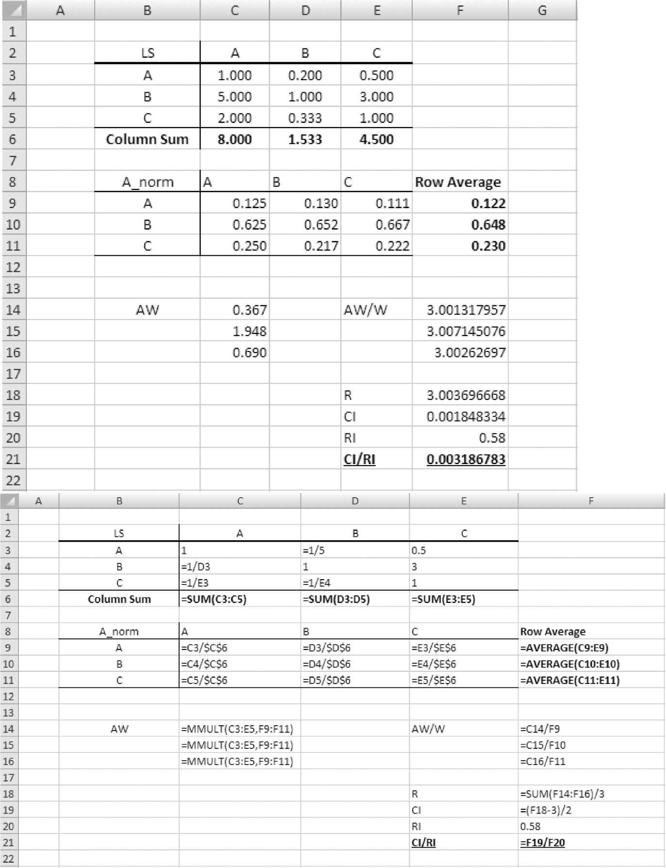
Illustration of AHP computation using Microsoft Excel (top image shows the AHP results and bottom image shows the Excel formula used to obtain the results).
AHP applies a hierarchical structure to assess decision-making problems for multiple decision criteria. The basic assumption of this hierarchical structure is that the attributes are homogeneous in terms of all the objectives. Another issue that needs to be mentioned here is that, for an effective application of AHP, it is important that the hierarchical structure includes only criteria that are independent, not redundant and additive ones. This ensures a valid comparison and high consistency of all the criteria. For dependent cases, the AHP framework should be modified using the feedback and supermatrix approaches (Rangone 1996).
6.7 Summary
In systems engineering design, resources are always limited, which requires system designers to constantly make decisions. Decision making is a process in which a decision maker must select one from a set of alternatives to achieve a specific goal. It is a selection process with some amount of information and usually involves some degrees of uncertainty. A decision-making problem can be solved by applying a six-step process: identify the problem, gather data, generate the alternatives, create an appropriate model based on the decision problem, compare the alternatives using the model, and finally execute the decision action.
In this chapter, we reviewed several decision-making models that are commonly applied in systems engineering, including decision making under risks and uncertainty. “Risks” implies that the likelihood of random future events can be estimated by probabilities, and “uncertainty” means that no knowledge of the future event’s probability can be obtained. On decision making under uncertainty, the Laplace, maximax, maximin, Hurwicz and minimax regret criteria were described; on decision making under risks, we introduced the expected value criterion.
The expected value criterion is considered risk neutral since the risks (probability) and expected value are linearly related; however, this might not capture the true behavior of humans. Different decision makers have different attitudes to risks; some may be risk averse and some may like taking risks (risk seeking). Von Neumann and Morgenstern’s utility theory provides a rigorous measure to incorporate attitudes to risk into the decision-making process. A decision maker’s attitude to risk can be obtained by having him/her choose the appropriate level of chance between receiving the best and worst possible payoff values. Using this concept, the utility of the decision maker with regard to a certain payoff value ri, denoted as u(ri), is the value of the probability qi, that makes the following two lotteries equivalent:

By defining the utility function, we use the expected utility value instead of the expected value to solve the decision-making problems that are involved with risks. Using the expected utility, we can easily choose between two lotteries by the following criteria:
The decision maker’s attitude to the risks can be assessed by looking at the risk premium (RP) value of the decision maker’s utility function. For a nondegenerate lottery, a decision maker is risk averse if and only if RP is positive, risk neutral if RP is zero, and risk seeking if RP is negative. Another way to derive this is to use the shape of the utility function; a strict concave utility function implies that the decision maker is risk averse, a strict linear function implies risk neutral, and a strict convex function implies risk seeking.
A decision tree is used to solve a decision-making problem with a sequence of decisions involved. There are two main constructs for developing a decision tree; the decision node and the event node. Once the decision tree is constructed, the expected value is calculated for each possible outcome and the decision is made by tracing the tree from the end events all the way back to the beginning of the decision tree; the optimal course of decision actions can thereby be obtained. The EVSI and EVPI values may be computed to evaluate feasibility when there is prior knowledge of a decision outcome.
In decision-making problems that involve multiple criteria/factors, the AHP method can be applied to rank the criteria and alternatives. AHP uses pairwise comparison between decision factors, and a four-step algorithm to develop normalized weightings for all the factors. To achieve valid comparison results, the consistency of the pairwise comparisons need to be checked to ensure the transitivity principle is satisfied. A CI can be computed for the pairwise comparison matrix and compared with an RI; if the ratio is less than 0.1, then the comparison can considered consistent, thus valid. An Excel template was presented at the end of the section to help readers to implement the AHP procedure efficiently.
Problems
- What is decision making? Why is decision making is important in systems engineering?
- What are the elements of decision making? Give an example of decision making and specify the elements of your example.
- What are the basic steps involved in making a decision?
- Discuss why using models is important when solving decision-making problems.
- A company is trying determine which project of five potential options to bid on to maximize profits. The payoff matrix is illustrated as follows (in thousands of dollars). The probabilities of the possible future events are shown above each future Fi in parentheses.
(0.10)
(0.30)
(0.15)
(0.20)
(0.25)
F1
F2
F3
F4
F5
A1
10
40
50
−20
30
A2
0
60
40
25
15
A3
−20
30
30
45
20
A4
20
50
10
50
35
A5
−15
20
35
15
10
From this payoff matrix, find
- Which alternative is dominated, so can be eliminated from the list?
- Which alternative should be chosen if we use the expected value criterion?
- Based on Problem 5, if the probabilities for all five futures are unknown, which alternative should be chosen based on
- The maximax criterion
- The maximin criterion
- The Laplace criterion
- The minimax regret criterion
- The Hurwicz criterion, if α = 0.20
- What is utility? Why is utility theory used to assess human decision-making behavior?
- If a utility function is
- u(x) = lnx
- u(x) = 2x + 3
- u(x) = x3
how would we choose between the following two lotteries?

and

- Calculate the RP for 8a, b, and c. Do these values imply a risk-seeking, risk-neutral or risk-averse decision maker?
- The human factors and systems (HFS) department is trying to determine which of two printers to purchase. Both machines will satisfy the department’s needs. Machine 1 costs $1500 and has a warranty contract, which, for an annual fee of $120, covers all the repairs. Machine 2 costs $2000, and its annual maintenance cost is a random variable. At the present time, the HFS department believes there is a 30% chance that the annual maintenance cost for Machine 2 will be $50, a 30% chance it will be $100, and a 40% chance it will be $150. Before the purchase decision is made, the department can have a certified technician evaluate the quality of Machine 2. If the technician believes that Machine 2 is satisfactory, there is a 70% chance that its annual maintenance cost will be $50, and a 30% chance it will be $100; if the technician believes that Machine 2 is unsatisfactory, there is a 20% chance that the annual maintenance cost will be $50, a 50% chance it will be $100, and a 30% chance it will be $150. Currently, it is expected that there is a 50% chance that the technician will give a satisfactory report, and the technician will charge $50. What should the HFS department do? What are the EVSI and EVPI? Construct a decision tree to help the HFS department find the correct solution.
- The human factors department at HFSCorp is trying to hire a regional manager for its newly opened branch in Daytona Beach, Florida. Based on the job duties and description, the hiring team has determined the following four criteria to make the selection: educational background (EB), prior experience (PE), references and recommendations (RR), and long-term career goal (CG). Since these criteria are not equally important to the job, the hiring team has made a pairwise comparison, as shown in the following matrix:
|
EB |
PE |
RR |
CG |
|
|
EB |
1.0 |
1/2 |
3.0 |
2.0 |
|
PE |
2 |
1.0 |
5.0 |
3.0 |
|
RR |
1/3 |
1/5 |
1.0 |
1.0 |
|
CG |
1/2 |
1/3 |
1.0 |
1.0 |
After screening a pool of applicants, the hiring team has narrowed down the selection to three candidates, Joe, Mike, and Anne. Based on the four criteria, the hiring team make a pairwise comparison matrix for each of the hiring criteria among the three candidates. For EB:
|
EB |
Joe |
Mike |
Anne |
|
Joe |
1.0 |
5 |
8 |
|
Mike |
1/5 |
1.0 |
3 |
|
Anne |
1/8 |
1/3 |
1.0 |
For PE:
|
PE |
Joe |
Mike |
Anne |
|
Joe |
1.0 |
1/4 |
1/2 |
|
Mike |
4 |
1.0 |
3 |
|
Anne |
2 |
1/3 |
1.0 |
For RR:
|
RR |
Joe |
Mike |
Anne |
|
Joe |
1.0 |
1/2 |
1/4 |
|
Mike |
2 |
1.0 |
1/3 |
|
Anne |
4 |
3 |
1.0 |
For CG:
|
RR |
Joe |
Mike |
Anne |
|
Joe |
1.0 |
2 |
1/3 |
|
Mike |
1 |
1.0 |
1/7 |
|
Anne |
3 |
7 |
1.0 |
Use AHP to help the hiring team decide which candidate to hire. Check the consistency for each of the matrices.