Chapter 9

Engineering Economy in Systems Engineering

In systems engineering, we are concerned with the efficient utilization of limited resources. There are two types of efficiency that systems designers need to take into account: technical efficiency and economic efficiency. In previous chapters, we have discussed the various types of systems technical performance measures, such as systems functionality, reliability, maintainability, and so on. On the other hand, we need to achieve the design technical objectives economically. Systems design requires capital investment, and every activity and effort occurring in the design requires resources, such as human labor and materials, and eventually these efforts are associated with cost. One of the most important goals in systems design is to minimize the cost involved and maximize the utility that is generated from the cost investment. Thus, designing for economic efficiency is very critical for systems engineering.

In systems engineering, we use the concepts of engineering economy to measure and control the cost involved in systems design and project management. Engineering economy is an applied economic science that addresses the economic issues within the engineering field. It is based on the principle of fundamental economics, and applying it in engineering design and related activities. The basis for the engineering economy is the time value of the money and opportunity cost. In this chapter, we will review some of the basic concepts of engineering economy and become familiar with the application of engineering economy in making decisions in systems engineering. More specifically, we will

1. Understand the concept of time value of the money and interest rate
2. Understand the concept of the present value (P), future value (F), annual equivalent value (A), and know how to convert from one to another
3. Describe how to use the values to compare different alternatives and make decisions
4. Introduce break-even analysis, based on the different values of money, and the decision-making process using break-even analysis

9.1 Interests and Time Value of Money

Time increases the value of money. We all know that if we deposit an amount of money in the bank, after a certain time, the amount deposited will increase. The bank pays interest on the money we deposit; this interest is paid for the time value of the deposited money. The reason that time increases the value of money is because money, as the general format of resources, can be invested to generate new values; for example, paying human labor for services provided, or investing in an engineering project to make more profit from it. We know that resources are limited; with money in hand, we can either consume now, or give the opportunity to someone else (i.e., the bank), so they can loan the money to someone who needs it to start a new project. Because we give up the opportunity of using the money now, and give the opportunity to others to use it first, in return, the opportunity we give needs to be compensated, in the form of interest.

What is interest? Interest is a fee paid by the borrower of the money (or asset) as compensation to its owner for the opportunity to use it. Interest can be considered as the price of borrowing the money. The amount of interest paid is determined by the interest rate and elapsed time for the borrowing of the money. We use i to denote the interest rate. The interest rate has to be specified according to the time it covers; for example, we need to specify whether it is the annual interest rate, monthly rate, or daily rate, as these rates of interest will be different.

There are two types of interest rate; namely, the simple interest rate and the compound interest rate. The simple interest rate, as the name implies, is simply the interest on the principal, and the interest earned will not generate further interest. For example, if the annual interest rate is a simple interest rate of 10%, for a deposit amount of $200, at the end of Year 1, the total amount in the bank account will be

$200+200\left(10\%\right)=\$220$

At the end of Year 2, since only the principal amount ($200) generates interest, we have

$220+200\left(10\%\right)=\$240$

and so on. With compound interest, on the other hand, the interest earned previously will generate future interest as well. So if 10% is the compound interest rate, at the end of Year 2, the total amount becomes

$220+220\left(10\%\right)=\$242$

If we denote the initial amount as x0 and the compound interest rate as i, then it is easy to derive the total amount xn after n years as

$x_n=x_0{\left(1+i\right)}^n$ (9.1)

The compound interest rate is that most commonly used for calculating the time value of money in the current economy; this is the interest rate we will be using in this chapter. Unless specified, the interest rate we refer to hereafter is the compound interest rate. With the concept of the interest rate, we can now measure the value of money between different points in time, or in other words, the equivalent worth of the money.

9.2 Economic Equivalence

In this section, we will be deriving the formulas for the equivalent money value for different points in time. Before we start, let us list all the terminologies and notions that will be used throughout the chapter.

N: Total time period: this can be years, months, weeks, days, and so on.

n: Time period: this can be years, months, weeks, days, and so on.

i: Interest rate per time period.

P: Present time equivalent value: This is the worth of the money at beginning of the time period, that is, n = 0; this value is also referred to as present worth, present value, or present equivalence.

F: Future time equivalent value: This is the worth of the money at end of a future period, that is, n ≥ 1; this value is also referred as future worth, future value, or future equivalence.

A: Annual equivalent value: This is the consecutive equal amount of the money’s worth at the end of each period. This value is also referred to as the annual worth or annual uniform worth/value of the money. One needs to pay attention here; although it is called the annual worth, it is actually the equal amount of the value at the end of the time period, so it could be the monthly equal amount if the time periods are measured in months.

With these notations being defined, we now can describe the formulas that can convert between the values of P, F, and A. In solving engineering economy problems, a useful method is to use graphical tools to illustrate the money flow on a timeline axis. We call this tool the money flow diagram, as illustrated in Figure 9.1.

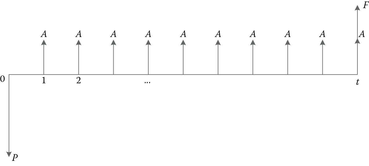
As shown in Figure 9.1, each of the time marks t represents the end of that period t, as we assume that money values are computed only at the end of that time period. If this money flow is a positive one (i.e., income or revenue), we draw the amount of the money using an upward arrow, to represent its positive value; if it is a negative one (i.e., investment, cost or loss), we draw the amount downward. By using the money flow diagram, we can visualize the profile of the money flow in a very intuitive way; thus, it is easier for us to carry out the analysis.

9.2.1 Present Value (P) and Future Value (F)

Let us first derive the relationship between the present value (P) and future value (F). A single amount of P occurs at the beginning of the time period (time = 0); what is the equivalent future value of F at the end of the time period n given the compound interest rate of i? The money flow diagram converting P to F is illustrated in Figure 9.2.

From Equation 9.1, it is easy to obtain the equation for converting P to F as

$F=P{\left(1+i\right)}^n$ (9.2)

We can use a factor to represent the relationship between P and F, written as

$F=P\left(\frac{F}{P}, i, n\right)$ (9.3)

The multiplier factor (F∕P,i,n) = (1 + i)n implies a conversion from P to F, given the values of n and i. From Equation 9.2, it is easy to find the reciprocal equation from F to P, written as in Equation 9.4,

$P=F\frac{1}{{\left(1+i\right)}^n}$ (9.4)

or

$P=F\left(\frac{P}{F}, i, n\right)$ (9.5)

with

$\left(\frac{P}{F}, i, n\right)=\frac{1}{{\left(1+i\right)}^n}$

Example 9.1

A deposit of $100 is made now, how much will it be worth after 10 years with an annual interest rate of 5%?

Solution: According to Equation 9.2, the total future amount of the deposit after 10 years is

$F=P{\left(1+i\right)}^n=100{\left(1+0.05\right)}^{10}=162.89\left(\text{USD}\right)$

In Appendix III of the book, the conversion factors have been precalculated for some of the most commonly used values of i and n, so readers can use the value directly from the tables for those i and n.

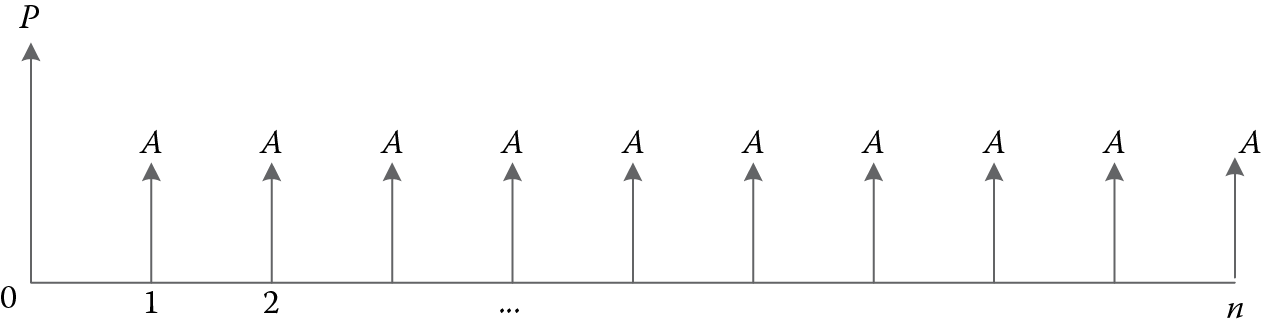
9.2.2 Annual Value (A) and Future Value (F)

The annual value is the equal amount of money that occurs at the end of each time period, starting at n = 1; its money flow diagram can be illustrated in Figure 9.3.

With the equal amount of A at the end of each time period, what is the equivalent future value F? From the money flow diagram, we can convert every A to the future value at n, starting from the last A, which occurs at n, all the way back to the first A, which occurs at n = 1. There are, in total, n − 1 time periods from the first occurrence to the last occurrence of A. So the future value of all the As can be obtained as follows:

$\begin{array}{c}F=A+A\left(1+i\right)+A{\left(1+i\right)}^2+A{\left(1+i\right)}^3+\cdots +A{\left(1+i\right)}^{n-1}\\ =A\left[1+\left(1+i\right)+A{\left(1+i\right)}^2+\cdots +A{\left(1+i\right)}^{n-1}\right]\end{array}$

Let

$S=1+\left(1+i\right)+{\left(1+i\right)}^2+\cdots +{\left(1+i\right)}^{n-1}$ (9.6)

So we have

$F=AS$

Multiplying by (1 + i) on both sides of Equation 9.6, we obtain

$\left(1+i\right)S=\left(1+i\right)+{\left(1+i\right)}^2+\cdots +{\left(1+i\right)}^n$ (9.7)

Subtracting Equation 9.6 from Equation 9.7, we have

$iS={\left(1+i\right)}^n-1$

We can obtain S by

$S=\frac{{\left(1+i\right)}^n-1}{i}$

So, substituting S back, we obtain Equation 9.8:

$F=A\frac{{\left(1+i\right)}^n-1}{i}$ (9.8)

or, we can say that the factor from A to F is

$\left(\frac{F}{A}, i, n\right)=\frac{{\left(1+i\right)}^n-1}{i}$ (9.9)

Similarly, the reciprocal of Equation 9.8 gives the formula of F to A, described in Equation 9.10:

$A=F\frac{i}{{\left(1+i\right)}^n-1}$ (9.10)

or

$\left(\frac{A}{F}, i, n\right)=\frac{i}{{\left(1+i\right)}^n-1}$ (9.11)

Example 9.2

If I deposit an equal amount of $100 every year for a time period of 20 years, with a compound interest rate of 5%, how much money will I have in total after 20 years?

Solution: From the problem description, we know that A = $100, i = 5% and n = 20 years. So, according to Equation 9.8, we can obtain the total amount future value by

$F=A\frac{{\left(1+i\right)}^n-1}{i}=100\frac{{\left(1+0.05\right)}^{20}-1}{0.05}=\$3306.60$

The factors of (A∕F,i,n) and (F∕A,i,n) are also precalculated in Appendix III for some of the most commonly used rates.

9.2.3 Annual Value (A) and Present Value (P)

This question related to A and P is very common as well; an example is when we purchase a house at a price of P, if we have a mortgage over n years at an interest rate of i, what is the annual equal payment of A? The relation between A and P is illustrated in Figure 9.4.

The formula for converting between A and P can be easily obtained by using the equations between A to F and P to F. From Equation 9.8 we have

$F=A\frac{{\left(1+i\right)}^n-1}{i}$

And from Equation 9.2, we know that

$F=P{\left(1+i\right)}^n$

Substituting Equation 9.2 in Equation 9.8 we have

$F=P{\left(1+i\right)}^n=A\frac{{\left(1+i\right)}^n-1}{i}$

$A=P\frac{i{\left(1+i\right)}^n}{{\left(1+i\right)}^n-1}$ (9.12)

or, we can say that the factor from P to A is

$\left(\frac{A}{P}, i, n\right)=\frac{i{\left(1+i\right)}^n}{{\left(1+i\right)}^n-1}$ (9.13)

The reciprocal of Equation 9.12 gives us the equation from A to P, as illustrated in Equation 9.14:

$P=A\frac{{\left(1+i\right)}^n-1}{i{\left(1+i\right)}^n}$ (9.14)

So, the factor from ? to P is

$\left(\frac{P}{A}, i, n\right)=\frac{{\left(1+i\right)}^n-1}{i{\left(1+i\right)}^n}$ (9.15)

Example 9.3

A house is sold for a cash price of $150,000; if the buyer has a loan for 30 years with zero down payment, with an interest rate of 4%, what is the annual mortgage payment?

Solution:

$P=\$150,000$

$i=4\%$

and

$n=30$

So, according to Equation 9.12,

$A=P\frac{i{\left(1+i\right)}^n}{{\left(1+i\right)}^n-1}=150,000\frac{4\%{\left(1+4\%\right)}^{30}}{{\left(1+4\%\right)}^{30}-1}=\$8,674.51$

The buyer needs to pay $8,674.51 every year for 30 years to pay off the mortgage.

The factors of (A∕P,i,n) and (P∕A,i,n) are also precalculated in Appendix III for some of the most commonly used rates.

Table 9.1 summarizes all the formulas described above. Readers may use it as a quick reference.

9.3 Decision Making Using Interest Formula

The interest formulas are very useful for decision making and comparing alternatives. When making decisions involving the time value of money, we have to keep in mind that

1. We need to convert the money occurring at different times into a common basis—in this case, converting to the same time point.
2. The decision should be the same regardless of the time point to which we choose to convert the time value of money. In other words, if we use the present value to find an alternative to be more favorable, then using the future value or the annual value should give us the same results. The “same results” means the same decision regarding which alternative is favorable. Whether we use P, F, or A as our criterion is solely dependent on the nature of the problem and complexity of the calculation for each value. We need to be flexible and choose one value that makes the calculation the easiest.

The decision-making process using the time value of money involves the following steps:

1. Determine the decision-making objective. Based on the problem, determine the objective of the decision making; usually the objective is to maximize income and minimize expenditure. If both income and expenditure are involved, then the objective is to maximize the overall net income (income minus cost).
2. Plot the money flow diagram for the problem. As mentioned earlier, the money flow diagram is a very useful tool for us to visualize the profile of the project to review the overall process of the project in terms of when the income and costs will occur and how much they will be, then facilitating the selection of the right value (present, future, or annual) as the common basis for comparison.
3. Based on the money flow diagram, select an equivalence value (present value, future value, or annual equal value) as the comparison basis. As we mentioned in the previous sections, no matter what value is being chosen, the decision should be the same (i.e., if the present value shows that one alternative is better, then the other two values should have the same comparison results, if no mistake is made in the conversion process). The criterion used for selecting the value should be based on the level of complexity of the computation and conversion of the time value. For example, if the majority of expenses occur in the present and at the end of the project period, then present value or future value equivalence should be used; if the projects have lots of annual equal money flow, then using the annual equal value may be a good idea. Although using a different criterion would give the same results, it could cause the calculation complexity to vary greatly.
4. Once the value of the criterion has been chosen, convert all the activities to the selected time value, by using the equation in Table 9.1 or from the interest factor table in Appendix III if the interest rate is listed there. Keep in mind that if both income and expenditure (costs) are involved, the convention is to use a positive sign for the income and a negative sign for the costs.
5. Based on the results for the converted value in step 4, select the alternative with the highest net profit, and make recommendations.

In the following section, we will use an example to illustrate how to use the formulas to compare alternatives and make decisions.

9.3.1 Present Value, Future Value, and Annual Value Comparison

Example 9.4

Company XYZ needs to install a cleaning system. There are currently two candidate systems that meet the basic requirements:

System 1: With an initial purchasing cost of $15,000, System 1 has a net save (value generated minus operation cost) of $2,000 annually. At the end of Year 4, System 1 will need a major overhaul, which will cost $1,500. The life span of System 1 is 8 years; after 8 years, System 1 will have a salvage value of $5,000.

System 2: With an initial purchasing cost of $25,000, system 2 has a net save of $3,300 annually. At the end of Year 4, System 2 will need a major overhaul, which will cost $2,500. The life span of System 2 is also 8 years; after 8 years System 2 will have a salvage value of $8,500.

With an interest rate of 5%, which system should be selected?

We will use present value, future value, and annual value to compare these two systems. Since the system has both positive incomes (i.e., the net save every year and salvage value) and negative costs (i.e., purchasing cost and overhaul cost), the goal of the decision making is to maximize the overall net income (income − costs). The money flow diagrams for System 1 and System 2 are illustrated in Figure 9.5.

9.3.1.1 Present Value Equivalence (PE) Criterion

Using the present value equivalence (PE) criterion, we need to convert all the activities to present value. By looking at Figure 9.5, it is obvious that, for example, for System 1, it includes a present cost of $15,000, a 4th year future cost of $1,500, an 8th year salvage value (income) of $5,000, and finally an annual equal save (income) of $2,000. System 2 has a similar cost and income structure. Knowing this structure, we can easily convert everything to present cost, shown as follows.

For System 1,

$\begin{array}{c}\text{PE}\left(1\right)=-15\text{,}000-1\text{,}500 \left(\frac{P}{F}, 5\%, 4\right)+2\text{,}000\left(\frac{P}{A}, 5\%, 8\right)+5\text{,}000\left(\frac{P}{F}, 5\%, 8\right)\\ =-15\text{,}000-1\text{,}500\left(0.8227\right)+2\text{,}000\left(6.463\right)+5\text{,}000\left(0.6768\right)=\$75.95\end{array}$

For system 2,

$\begin{array}{c}\text{PE}\left(2\right)=-25\text{,}000-2\text{,}500 \left(\frac{P}{F}, 5\%, 4\right)+3\text{,}300\left(\frac{P}{A}, 5\%, 8\right)+8\text{,}500\left(\frac{P}{F}, 5\%, 8\right)\\ =-25\text{,}000-2\text{,}500\left(0.8227\right)+3\text{,}300\left(6.463\right)+8\text{,}500\left(0.6768\right)=\$23.95\end{array}$

Since PE(1) > PE(2), system 1 should be selected when the interest rate is 5%.

9.3.1.2 Future Value Equivalence (FE) Criterion

Using the future value as the comparison basis, we need to convert everything into the future time value, as follows.

For System 1,

$\begin{array}{c}\text{FE}\left(1\right)=-15\text{,}000\left(\frac{F}{P}, 5\%, 8\right)-1\text{,}500\left(\frac{F}{P}, 5\%, 4\right)+2\text{,}000\left(\frac{F}{A}, 5\%, 8\right)+5\text{,}000\\ =-15\text{,}000\left(1.477\right)-1\text{,}500\left(1.216\right)+2\text{,}000\left(9.549\right)+5\text{,}000\\ =\$119.00\end{array}$

For System 2,

$\begin{array}{c}\text{FE}\left(2\right)=-25\text{,}000\left(\frac{F}{P}, 5\%, 8\right)-2\text{,}500\left(\frac{F}{P}, 5\%, 4\right)+3\text{,}300\left(\frac{F}{A}, 5\%, 8\right)+8\text{,}500\\ =-25\text{,}000\left(1.477\right)-2\text{,}500\left(1.216\right)+3\text{,}300\left(9.549\right)+8\text{,}500\\ =\$46.70\end{array}$

And again, FE(1) > FE(2); the decision-making result is the same as that using the PE criterion.

9.3.1.3 Annual Value Equivalence (AE) Criterion

Using the annual value equivalence (AE) criterion, everything needs to be converted to an annual equal amount, shown as follows.

For System 1,

$\begin{array}{c}\text{AE}\left(1\right)=-15\text{,}000\left(\frac{A}{P}, 5\%, 8\right)-1\text{,}500\left(\frac{P}{F}, 5\%, 4\right)\left(\frac{A}{P}, 5\%, 8\right)\\ +2\text{,}000+5\text{,}000\left(\frac{A}{F}, 5\%, 8\right)\\ =-15\text{,}000\left(0.1547\right)-1\text{,}500\left(0.8227\right)\left(0.1547\right)+2\text{,}000+5\text{,}000\left(0.1047\right)\\ =\$12.09\end{array}$

For System 2,

$\begin{array}{c}\text{AE}\left(2\right)=-25\text{,}000\left(\frac{A}{P}, 5\%, 8\right)-2\text{,}500\left(\frac{P}{F}, 5\%, 4\right)\left(\frac{A}{P}, 5\%, 8\right)\\ +3\text{,}300+8\text{,}500\left(\frac{A}{F}, 5\%, 8\right)\\ =-25\text{,}000\left(0.1547\right)-2\text{,}500\left(0.8227\right)\left(0.1547\right)+3\text{,}300+8\text{,}500\left(0.1047\right)\\ =\$4.27\end{array}$

For this problem, it is easy to see that using AE is a little more complex than PE and FE. This is mainly because that the overhaul cost that occurs in the middle of the life span needs to be converted to either present or future value first before it can be converted to the annual value.

9.3.2 Rate of Return

The rate of return is another important measure of value besides the time value of money measures. In some situations, the rate of return is believed to be the best evaluation criterion for comparing alternatives, as it does not rely on the external interest rate, but rather represents the cost-benefit value of the money flow. Rate of return is defined as the interest rate i* that causes the two alternatives to be the same, or

${\text{PE}}_1\left(i\text{*}\right)={\text{PE}}_2\left(i\text{*}\right)$

or

${\text{FE}}_1\left(i\text{*}\right)={\text{FE}}_2\left(i\text{*}\right),{\text{AE}}_1\left(i\text{*}\right)={\text{AE}}_2\left(i\text{*}\right)$

Rate of return is also considered as a universal measure as it gives us the interest rate that makes the alternatives equal, and we can use rate of return as a threshold to compare with the current interest rate to make decisions. As the market interest rate changes, the rate of return does not change; thus, we can adjust the decision made according to the new market rate, without going through the calculation again; while using other criteria, every time the market rate changes, a new calculation is needed as the result will change. The rate of return is also useful for projects that have different life cycles; it serves as the only criterion by which to compare them.

Let us use Example 9.4 to show how to obtain the rate of return. As mentioned above, the rate of return i* is the interest rate that satisfies

${\text{PE}}_1\left(i\text{*}\right)={\text{PE}}_2\left(i\text{*}\right)$

or

${\text{PE}}_1\left(i\text{*}\right)-{\text{PE}}_2\left(i\text{*}\right)=0$

This is obviously a high-order nonlinear equation, and it would be difficult to obtain the analytical solution unless applying some numerical analysis. Here we use an approximation technique called linear interpolation. Using this technique, we find two points that make the results change sign. It is assumed that if the two points are close enough, then a straight line can be used to approximate the curve connecting these two points. Since the two rates make PE1(i*) − PE2(i*) change sign (either from positive to negative or vice versa), then the line will intersect PE1(i*) − PE2(i*) = 0 and the intersection point will be the rate of return.

Example 9.5

From the previous calculation, we know that with i = 5%, PE(1) − PE(2) = 75.95 − 23.95 = +52.

We then use i = 2% to recalculate the new present value again.

At a 2% interest rate,

$\begin{array}{c}\text{PE}\left(1\right)=-15\text{,}000-1\text{,}500 \left(\frac{P}{F}, 2\%, 4\right)+2\text{,}000\left(\frac{P}{A}, 2\%, 8\right)+5\text{,}000\left(\frac{P}{F}, 2\%, 8\right)\\ =-15\text{,}000-1\text{,}500\left(0.9238\right)+2\text{,}000\left(7.325\right)+5\text{,}000\left(0.8535\right)=2\text{,}431.80\end{array}$

$\begin{array}{c}\text{PE}\left(2\right)=-25\text{,}000-2\text{,}500 \left(\frac{P}{F}, 2\%, 4\right)+3\text{,}300\left(\frac{P}{A}, 2\%, 8\right)+8\text{,}500\left(\frac{P}{F}, 2\%, 8\right)\\ =-25\text{,}000-2\text{,}500\left(0.9238\right)+3\text{,}300\left(7.325\right)+8\text{,}500\left(0.8535\right)=4\text{,}117.75\end{array}$

$\text{PE}\left(1\right)-\text{PE}\left(2\right)=-1\text{,}585.95$

So, clearly, the rate of return is between 2% and 5% since PE(1) − PE(2) has changed sign. We apply linear interpolation, illustrated in Figure 9.6.

Since it is linear, the following equation holds:

$\frac{i\text{*}-2\%}{5\%-2\%}=\frac{0-\left(-1585.95\right)}{52-\left(-1585.95\right)}$

so

$i\text{*}=2\%+3\%\frac{1585.95}{1637.95}=4.9\%$

So, at an interest rate of 4.9%, the two systems will yield the same result. When the interest rate is larger than the rate of return level, the system with less initial cost will be more desirable, since with a higher interest rate, the higher the initial cost, the greater impact it will have on the overall cost throughout the life cycle. We can also say that with a greater interest rate, the initial cost will generate more interest; if we need to borrow the money, it would be more expensive, and thus leaves the higher initial cost as the less desirable option. When the interest rate is less than the rate of return, the system with the higher initial cost will be the better choice.

From the results, we can see in the original question that the market interest rate is 5% > i*; this means that System 1 (with lower initial cost) will outperform System 2 (with higher initial cost).

9.4 Break-Even Analysis

Decisions made in systems engineering are primarily based on predictions of future events; engineers use current understanding of the systems design project and its anticipated future environment to estimate the economic benefits for the system to be designed. However, due to various levels of uncertainty that are involved in the decision factors in economic analysis, the estimation of the cost and benefits have various levels of uncertainty and risk. Examples of these factors include global and local political and economic situations, technological advancement, and the limitations of economic analysis methods and models. We have addressed decision-making uncertainty and risks in previous chapters; some of the models can certainly be used in engineering economy analysis to address these. In dealing with uncertainty in systems design, there is no guarantee that a project estimation will be accurate; what can be done is to provide a bigger picture to incorporate the risk and uncertainty factors into consideration, providing different scenarios or baselines for decision makers to deal with unexpected risks in the future. Generally speaking, there are several ways that a systems designer can prepare for future risks/uncertainty:

1. Provide break-even analysis to illustrate the relationship between costs, profits, and quantities, finding the break-even points for these factors, thus enabling decision makers to develop an overall picture of the profitability of the project.
2. Develop a sensitivity analysis model; by using “what-if” scenarios in the model, major uncertainties and risks can be anticipated. In sensitivity analysis, the range from the best-case to the worst-case scenario can be covered, enabling decision makers to develop strategies for possible upcoming scenarios. When one of these scenarios occurs, a corresponding strategy can be applied with confidence.

   Break-even analysis has been used widely in business operation management; in this section, we shall use some examples to illustrate how to conduct a break-even analysis for business decisions.

   9.4.1 Cost Volume Break-Even Analysis

   In product design and capacity planning, we need to focus on the relationship between costs (fixed and variable), revenue, and production volume. In product design, if there is a fixed cost involved, then the product volume must achieve a certain level to break even.

   Example 9.5

   Company XYZ is adding a new assembly line. Investing in the new line requires a monthly payment of $10,000, the cost of the parts that the new assembly line produces is $10, and they are sold for a price of $35 per piece. Assuming all parts can be sold, how many parts must be assembled per month to break even?

   Solution: In this problem the fixed cost (FC) per month is $10,000, the variable cost (VC) is $10 per piece and the revenue (R) is $35 per piece, so the break-even volume (Q) is determined by the point at which the total monthly profit breaks even with the fixed cost, shown as follows:

   $\text{FC}=Q\left(R-\text{VC}\right)$ (9.16)

   or

   $Q=\frac{\text{FC}}{R-\text{VC}}$ (9.17)

   So, the break-even volume is

   $Q=\frac{10,000}{35-10}=400$

   Company XYZ must sell at least 400 pieces per month to break even.

   9.4.2 Rent-or-Buy Break-Even Analysis

   Sometimes, system designers face the decision of renting a resource or buying it; this is similar to the cost volume analysis above, if we treat the purchasing cost as the fixed cost for the resource.

   Example 9.6

   An automobile can be purchased at $15,000 and lasts 10 years. After 10 years, the automobile can be sold at $2,000. The annual operation and maintenance cost is $400.

   As an alternative, the same automobile can be leased at the rate of $50 per day. For how many days each year may the automobile be used for these two options to break even?

   Solution: If we denote the break-even number of days as N, then the average annual cost of owning a vehicle equals the annual renting cost, that is,

   $15,000\left(\frac{A}{P}, 10\%, 10\right)-2,000\left(\frac{A}{F}, 10\%, 10\right)+400=50N$

   $15,000\left(0.1627\right)-2,000\left(0.0627\right)+400=50N$

   $2715.1=50N$

   $N\cong 55 \left(\text{days}\right)$

   So, the number of days to break even with the annual cost is 55 days.

   The above question can also be asked in a different way: What is the minimum number of days of usage of the vehicle to make purchasing it more desirable? We have given readers some exercises at the end of the chapter to practice.

   9.5 Summary

   Systems design requires systems to be developed in an efficient manner, both technically and economically. In this chapter, basic concepts and measures for systems engineering economy were reviewed. The key concept in engineering economy is the time value of money. Time will increase the value of a money amount. Since monetary activities occur throughout the whole system life cycle, this requires us to analyze and compare the alternatives from a common time basis. In this chapter, we reviewed three fundamental time values of money: present value equivalence (PE), future value equivalence (FE), and annual value equivalence (AE); the formulas to convert between these values were derived and summarized. We used some examples to illustrate how to use these three values as criteria for the basis to compare multiple alternatives. As a universal measure, the rate of return criterion was also presented. At the end of the chapter, we introduced the break-even model in economic analysis; two examples, volume of production and rent-or-buy, were used to illustrate this analysis method. Break-even analysis provides a reference point for decision makers to relate costs and profits, providing a baseline for determining the profitability of the project. We need to keep in mind that the material covered in this chapter is very basic in nature; engineering economy is a big subject that itself needs a textbook to cover. For more in-depth review, readers can refer to any other engineering economy books that provide a comprehensive coverage of the subject.

   Problems

3. Explain why economic analysis is important in systems engineering.
4. What is interest? Compare the simple interest rate and the compound interest rate.
5. When taking a loan from the bank, there are two options. Option 1: the annual interest rate is 8%, compounded monthly. Option 2: the annual interest rate is 15%, compounded quarterly. Which option should the borrower choose?
6. How many years does it take for a deposited sum to double itself, given the interest rate of 10%, compound annually?
7. What annual compound interest rate is necessary for a deposit to triple itself in 10 years?
8. Assuming that the interest rate is 5%, compounded annually,
   1. What is the present equivalent value of an overhaul cost of $2,000 that will occur 5 years from now?
   2. The initial investment is $20,000. What is the annual equal amount of saving over the 5-year period to justify this investment?
9. The same amount of money occurs at different time points; the amount occurring first has a higher equivalent value than the one occurring next. Is this statement true or false? Justify your answer.
10. A company has a loan of $150,000; the annual compound interest rate is 5%. The company begins to pay back the loan at the end of the first year, at an equal amount, and hopes to pay it off after 10 years. What is the annual equal amount of the payment?
11. In Problem 8, if there were no payment for the first year, and the company started to pay the loan back at the end of the second year, and paid it off after 10 years, what is the annual equal amount of the payment?
12. The HFS department is considering two computer servers for their lab. Server A costs $7,000 initially and has a salvage value of $1,500 after 10 years; Server B costs $5,000 initially and has a salvage value of $1,000 after 10 years. Assuming that they both satisfy the needs of the department, with an annual compound interest rate of 6%, which server should be chosen?
13. For a 5-year investment project, the initial investment at time 0 is $100,000, and the investment at beginning of the second year is $80,000. The annual revenue after the second investment is $50,000 (from Year 2 to Year 5); the salvage value after Year 5 is $70,000. Assuming an annual compound interest rate of 5%, should this project be invested in?
14. Calculate the rate of return for the project in Problem 11. (Hint: the rate of return makes the net value of the project equal 0.)
15. The following table shows the money flow for a project, with i = 10%, compounded annually.

    Year	0	1	2	3	4	5
    Money flow	−1000	200	250	250	250	250

    Is this project feasible?

16. A company is planning to build a 10,000 sq. ft. warehouse in 3 years. Option 1 is to buy a piece of land for $80,000 and build a temporary warehouse on it, the cost of which is $70/sq. ft.; after 3 years, it is estimated that the company can sell the land for $90,000, and sell the warehouse for $120,000. Option 2 is to rent a warehouse. The annual rent is $150/sq. ft., to be paid annually. The annual compound interest rate is 10%. Which option should the company take? Draw the money flow diagram and solve it using the PE, FE, and AE criteria.
17. A person borrows $20,000 at the beginning of Year 1. Every year he is required to pay $4,000 so that the loan is paid off after 10 years. What is the annual compound interest rate? (Hint: use linear interpolation.)
18. Company XYZ is considering buying new power supply equipment. Currently there are two types of equipment are under consideration. Type A: the initial cost is $14,000, the salvage value is $2,000 after 4 years, the hourly cost is $0.84/h, and the annual maintenance fee is $1,200. Type B: the initial cost is $5,500, there is no salvage value after 4 years, and the hourly cost is $0.67/h plus a human labor fee of $0.80/h. Assuming that the interest rate is 10%, compounded annually, how many hours per year does the equipment need to be used to make the two types break even?
19. A company has a production capacity of 50,000 tons annually; the annual fixed cost is $8,000,000, the sale price for each ton is $1,500, tax and other costs are 10% of the sale price, and the variable cost is $1,150/ton. What is the annual percentage of the production capacity required to make it break even?