Chapter 7

System Optimization Models

Systems engineering is concerned with designing complex systems in an efficient and economic manner. No matter what types of systems are being developed, resources nevertheless have to be consumed; these resources could be human power, capital funds, raw materials, or working hours, to name a few. All resources are limited; as system engineers, we need to obtain the best value from these limited resources, or optimize their utilization. Systems engineering needs to incorporate optimization to achieve the design objectives. As a matter of fact, systems engineers carry out optimization on an almost daily basis; for example, we can think of decision making as a kind of optimization, as we need to pick the best alternatives to achieve the optimum outcome. The optimization methods and models we review in this chapter are more general, and these methods and models originate from operations research.

In this chapter, we will present a high-level introduction to optimization problems and the application of optimization models in systems engineering. Optimization is defined within the systems engineering context, and since this is not an operations research (OR) textbook, we will focus on the two most commonly used optimization models in systems design: unconstrained classic models and constrained optimization based on mathematical programming. More specifically, in this chapter, we will

1. Give a formal definition of optimization and its fundamental characteristics and features. We will give a general mathematical formulation for optimization problems.
2. Review the classic unconstrained optimization model. This type of model is based on calculus operations; some basic concepts will be reviewed.
3. Review constrained optimization models using mathematical programming. More specifically, we will focus on the basic model of mathematical programming, the linear programming (LP) model. We will discuss the formulation process and solutions of LP models based on graphical methods (two decision variables) and the Simplex algorithm, using software (i.e., Excel) to solve them.

This chapter will give an overview of the fundamental concepts of optimization that are commonly used in systems engineering problem solving, giving readers a good starting point and correct mindset for optimization formulations in complex system designs.

7.1 What Is Optimization?

As mentioned earlier, optimization is one of the most important topics in the area of applied mathematics, particularly in operations research. Optimization seeks the value of certain factors or variables to optimize the objective function value (maximization or minimization). In the simplest case, optimization is a mathematical model/algorithm/procedure to determine the value of the input variables with regard to some constraints to achieve optimal system performance, often measured as the value of an objective function(s). Optimization is a critical part of OR; many branches of OR fall under optimization, such as mathematical programming, combinatorial optimization, queuing theory, decision making, game theory, engineering design and control, and so on.

We should mention here that the generalized theory of optimization differs from the decision-making models we discussed in Chapter 6. In optimization theory, the goal is to find the decision variable values from a defined domain to optimize the objective function. Compared to decision-making theory, in which we have a limited number of activities to choose from, the possible values for decision variables in optimization problems are often from sets/domains that have unlimited values (e.g., from a continuous real interval value). One usually cannot find the solution by enumerating all the possible values into the objective functions.

We can use the following expression to define a general optimization problem:

Given a function f : A→ℝ, where A is the subset of Euclidean space ℝn, and ℝ is a real number, we seek an element x0 ∈ A, such that f(x0) ≤ f(x) for any x in A or ∀x ∈ A for a minimization optimization; or f(x0) ≥ f(x) for any x in A or ∀x ∈ A for a maximization optimization.

Optimization methods and models were developed together with calculus long ago, but only in recent years, especially after the 1940s, did they start to bloom and undergo rapid development and application, due to increased demand from the advancement of computer technology, large complex system development and design, and the accelerating speed of product turnover, which made optimization a feasible tool for solving many of these problems. The application of optimization also drives the development of the theory, which led to more advancement of the OR field.

7.2 Unconstrained Optimization Models

In this section, we will introduce the basic concepts of unconstrained optimization by differentiation. Function optimization is the fundamental application of differentiation, which is covered by any first-year college calculus textbook. For readers to understand the concepts better, we give a brief overview of the basic differentiation concepts. Please keep in mind that this review is by no means comprehensive. For a more in-depth review of differentiation calculus, please see a textbook such as Single Variable Calculus by James Stewart (7th edn).

7.2.1 Derivatives and Rate of Change

In calculus, the derivative at a certain point is the rate of change of the function with respect to its input variable at that point. For example, a function y = f(x) at the point (x0,y0)’s rate of change is the slope of the tangent line that passes the point (x0,y0), as shown in Figure 7.1. Using the formal definition of a limit, we have the following definition for the slope (provided that this limit exists).

$\text{slope}=\underset{x\to x_0}{\lim }\frac{f\left(x\right)-f\left(x_0\right)}{x-x_0}$ (7.1)

For example, the slope at x = 2 for function y = f(x) = x2 + 3x is

$\begin{array}{l}\underset{x\to 2}{\lim }\frac{x^2+3x-2^2-3\left(2\right)}{x-2}\\ =\underset{x\to 2}{\lim }\frac{x^2+3x-2^2-3\left(2\right)}{x-2}\\ =\underset{x\to 2}{\lim }\frac{x^2-2^2+3\left(x-2\right)}{x-2}\\ =\underset{x\to 2}{\lim }\left[\left(x+2\right)+3\right]=4+3=7\end{array}$

Using the idea of limits, we can define the derivative as follows: The derivative of a function f at the value of x, denoted as f′(x), is defined as

$f^{\prime }\left(x\right)=\underset{h\to 0}{\lim }\frac{f\left(x+h\right)-f\left(x\right)}{h}$ (7.2a)

provided that the above limit exists.

Another equivalent way to define the derivative is

$f^{\prime }\left(x\right)=\underset{a\to x}{\lim }\frac{f\left(a\right)-f\left(x\right)}{a-x}$ (7.2b)

As another notation for f′(x), it can sometimes also be written in the following format:

$y=f\left(x\right)$

$f^{\prime }\left(x\right)=\frac{\text{d}y}{\text{d}x}$

As a prerequisite, we assume that readers have a basic understanding of derivatives, so we will not spend too much time on deriving the derivative functions; here we just list the formulas for the most commonly used functions, as the derivatives for other functions can be derived from a combination of these common formulas.

1. Derivative of the constant c

   $y=f\left(x\right)=c, f^{\prime }\left(x\right)=\frac{\text{d}y}{\text{d}x}=0$ (7.3)

   Furthermore, if c is a constant and y = cf(x), then

   $\frac{\text{d}y}{\text{d}x}=c{f}^{\prime }\left(x\right)$ (7.4)

2. Derivative of power functions

   $y=f\left(x\right)=x^n, f^{\prime }\left(x\right)=\frac{\text{d}y}{\text{d}x}=n{x}^{n-1}$ (7.5)

3. The sum/subtract rule:

   If f(x) and g(x) are both differentiable, and h(x) = f(x) ± g(x), then

   $h^{\prime }\left(x\right)=f^{\prime }\left(x\right)\pm g^{\prime }\left(x\right)$ (7.6)

4. The product rule:

   If f(x) and g(x) are both differentiable, and h(x) = f(x) g(x), then

   $h^{\prime }\left(x\right)=f^{\prime }\left(x\right)g\left(x\right)+f\left(x\right)g^{\prime }\left(x\right)$ (7.7)

5. The quotient rule:

   If f(x) and g(x) are both differentiable, and h(x) = f(x)∕g(x), then

   $h^{\prime }\left(x\right)=\frac{g\left(x\right)f^{\prime }\left(x\right)-f\left(x\right)g^{\prime }\left(x\right)}{{\left[g\left(x\right)\right]}^2}$ (7.8)

6. Derivatives of trigonometric functions

   $y=f\left(x\right)=\sin \left(x\right),f^{\prime }\left(x\right)=\cos (x)$ (7.9)

   $y=f\left(x\right)=\cos \left(x\right),f^{\prime }\left(x\right)=-\sin \left(x\right)$ (7.10)

   $y=f\left(x\right)=\tan \left(x\right),f^{\prime }\left(x\right)={\sec }^2\left(x\right)$ (7.11)

7. The chain rule:

   If g is differentiable at x and f is differentiable at g(x), then the derivative for the composite function y = f[g(x)] is given by

   $\frac{\text{d}y}{\text{d}x}=f^{\prime }\left[g\left(x\right)\right]g^{\prime }\left(x\right)$ (7.12)

8. Some special functions:

$y=f\left(x\right)=e^x, f^{\prime }\left(x\right)=e^x$ (7.13)

$y=f\left(x\right)=\ln \left(x\right),f^{\prime }\left(x\right)=\frac{1}{x}$ (7.14)

Using the above basic derivatives functions, we can solve some derivative-related problems. For example, in economics, the concept of marginal cost is defined as the instantaneous rate of change of the total cost function, or the first-order derivative of the total cost function C(x); the marginal cost function is dC(x)∕dx, or C′(x). Suppose that a company has estimated the cost function of producing x items is as follows:

$C\left(x\right)=0.05x^2+50x+1000$

The marginal cost function (or rate of change function) is given by the first-order derivative

$C^{\prime }\left(x\right)=\frac{\text{d}C\left(x\right)}{\text{d}x}=\frac{\text{d}\left(0.05x^2\right)}{\text{d}x}+\frac{\text{d}\left(50x\right)}{\text{d}x}+\frac{\text{d}\left(1000\right)}{\text{d}x}=0.1x+50$

The marginal cost at x = 100 items is

$C^{\prime }\left(100\right)=0.1\left(100\right)+50=60\left(\text{\$ per item}\right)$

If the function has more than one independent variable, that is, y = f(x1, x2,…, xn), to find the rate of change, we need to use partial differentiation. The process of partial differentiation is that all other variables except for the variable of interest are treated as constant, and the differentiation procedure is exactly the same as the single-variable function. The partial differentiation is denoted as ∂y∕∂x. For example,

$y=f\left(x_1,x_2\right)=4x_1^2+5x_1{x}_2+6x_2^3+8$

The partial differentiation of y with respect to x1 is

$\frac{\partial y}{\partial x_1}=8x_1+5x_2$

And the partial differentiation of y with respect to x2 is

$\frac{\partial y}{\partial x_2}=5x_1+18x_2^2$

For a more comprehensive review of partial differentiation and related concepts, readers please refer to any calculus textbook such as Calculus by James Stewart (2011).

Understanding the basic concept of derivatives, we now see how derivatives can help us to find the optimal (maximum or minimum) value. Let us first look at the function values around the optimum points. We denote a as the local minimum point if and only if f(a) ≤ f(x), for all x around c, as illustrated in Figure 7.1.

Similarly, we define b as the local maximum point if and only if f(b) ≥ f(x) for all x around b, as illustrated in Figure 7.2.

From Figure 7.1 and Figure 7.2, one can easily see that the tangent line at the local minimum or maximum is horizontal; or, using derivatives, we have f′(a) = 0, and f′(b) = 0. This is the necessary condition for the local optimum, as described in Fermat’s theorem.

Local Optimum Theorem (or Fermat’s Theorem)

If function f has a local minimum or maximum at c, and if the first-order derivative of f exists, then f′(c) = 0.

The condition f′(c) = 0 is only necessary for an optimum point, but not sufficient, because if a function y = f(x) is differentiable at point x = c, and f′(a) = 0, the c could be a minimum or maximum, or another possibility is that c is a point of reflection (a horizontal line at c). In order to determine whether it is a minimum or maximum, we must look at the second-order derivative. For the local minimum point x = c, for the value less than c, the rate of change is negative, until it reaches zero at x = c, and then it starts to increase (becoming positive); the rate of change of the rate of change is positive (Figure 7.1), or f″(c) > 0; for the local maximum point, we can easily see from Figure 7.2 that the rate of change of the rate of change at the maximum point is negative, or f″(c) < 0. If the second-order derivative is still zero, then a higher-order derivative is sought until a nonzero value is found at the nth-order derivative. Then a similar rule applies to determine the optimum point:

$x=c\text{is the local minimum if}{f}^{\left(n\right)}\left(c\right)>0\text{, }n\text{ is even}$

$x=c\text{is the local minimum if}{f}^{\left(n\right)}\left(c\right)<0\text{, }n\text{ is even}$

$x=c\text{is the point of reflection if}{f}^{\left(n\right)}\left(c\right)=0\text{, }n\text{ is odd}$

For functions y = f(x1, x2,…, xn) with more than one independent variable, the necessary condition that the point x* = [x1, x2,…, xn] is a stationary point is that the first-order partial derivative at x* equals zero, or,

$\left[\frac{\partial y}{\partial x_1}, \frac{\partial y}{\partial x_2}, \dots , \frac{\partial y}{\partial x_n}\right]=0$ (7.15)

To determine whether x* is the local minimum or maximum, the second-order partial derivatives are similarly required; namely, the Hessian matrix, which is derived as

$H\left(f\right)=\left[\begin{array}{cccc}\frac{{\partial }^{2}f}{\partial x_1^2}& \frac{{\partial }^{2}f}{\partial x_1\partial x_2}& \dots & \frac{{\partial }^{2}f}{\partial x_1\partial x_n}\\ \frac{{\partial }^{2}f}{\partial x_2\partial x_1}& \frac{{\partial }^{2}f}{\partial x_2^2}& \dots & \frac{{\partial }^{2}f}{\partial x_2\partial x_n}\\ \dots & \dots & \dots & \dots \\ \frac{{\partial }^{2}f}{\partial x_n\partial x_1}& \frac{{\partial }^{2}f}{\partial x_n\partial x_2}& \dots & \frac{{\partial }^{2}f}{\partial x_n^2}\end{array}\right]$ (7.16)

If the determinant of H(f(x*) or |H(f(x*)|>0, then x* = [x1, x2,…, xn] is a minimum point and if |H(f(x*)| < 0, then x* = [x1, x2,…, xn] is a maximum point.

As mentioned earlier, in systems engineering, we often need to put limited resources to the best use; differentiation-based optimization is one of the most commonly used models to find the lowest cost, maximum profit, least use of materials, and so on. Let us see how we can use the above conditions to solve an optimization problem.

Example 7.1

Imagine that we are trying to build a cylindrical container. The container is required to have a volume of V. What is the radius of the base circle (r) that uses the minimum amount of materials to build the cylinder? What is the ratio of the height h to r?

Solution: A cylinder is shown in Figure 7.3. If we ignore the thickness of the materials, the amount of the materials to build the cylinder can be represented by the area of the cylinder. Let us denote the area of the cylinder as S, and the height of the cylinder is h, and assume that the container is sealed, so we have the following formula for the total area:

$S\left(r\right)=2\pi r^2+2\pi rh$

because

$V=\pi r^{2}h$

so

$h=\frac{V}{\pi r^2}$

Substituting into the formula for the total area, we have

$S\left(r\right)=2\pi r^2+2\frac{V}{r}$

S(r) is continuous and differentiable, so applying the theorem of optimization, we obtain the following equation

$S^{\prime }\left(r\right)=4\pi r-2\frac{V}{r^2}=0$

Solving the above equation, we have

$r=\sqrt[3]{\frac{V}{2\pi }}$

To verify that this is truly the minimum value, we use the second-order derivative as follows:

$S^{″}\left(r\right)=4\pi +4\frac{V}{r^3}>0$

so it is truly a minimum value.

$\frac{h}{r}=\frac{\frac{V}{\pi r^3}}{r}=\frac{V}{\pi r^3}=\frac{V}{\pi \frac{V}{2\pi }}=2$

The ratio h/r = 2 when materials used are minimum.

Let us look at an example that involves multiple independent variables: f(x,y,z) = x2 + 2y2 + 3z2 + 2x + 4y − 12z. First, apply the necessary condition to find the stationary point:

$\{\begin{array}{c}\frac{\partial f}{\partial x}=2x+2=0\\ \\ \frac{\partial f}{\partial y}=4y+4=0\\ \\ \frac{\partial f}{\partial z}=6z-12=0\end{array}$

So, we can obtain the stationary point as (−1, −1, 2).

Next, we need to derive the Hessian matrix by taking the secondary partial derivative as follows:

$\frac{{\partial }^{2}f}{\partial x^2}=2, \frac{{\partial }^{2}f}{\partial x\partial y}=0, \frac{{\partial }^{2}f}{\partial x\partial z}=0$

$\frac{{\partial }^{2}f}{\partial y\partial x}=0, \frac{{\partial }^{2}f}{\partial y^2}=4, \frac{{\partial }^{2}f}{\partial y\partial z}=0$

$\frac{{\partial }^{2}f}{\partial z\partial x}=0, \frac{{\partial }^{2}f}{\partial z\partial y}=0, \frac{{\partial }^{2}f}{\partial z^2}=6$

So, the Hessian matrix is

$H=\left[\begin{array}{ccc}2& 0& 0\\ 0& 4& 0\\ 0& 0& 6\end{array}\right]$

and it is easy to see that |H|>0, so f(x, y, z) reach the minimum point at (−1, −1, 2), fmin = −15.

7.3 Constrained Optimization Model Using Mathematical Programming

With most of the optimization problems with which engineering design is concerned, the resources are often limited. Such resources could be human labor hours, capital funds, materials, or equipment. As system designers, we need to seek the optimal utilization of the limited resources such as maximizing the profit; or, sometimes, when the objectives of the system are set, we need to seek the most optimal planning of production or scheduling of labor to minimize the cost. For example, a production schedule would want to maximize weekly profit by producing as many items as possible, but the schedule is subject to the limited raw materials, the workforce, and the working hours available per week. Similar examples may also be found choosing between different investments that have alternative payment schedules, or work-schedule problems to meet certain days’ requirements yet minimizing the number of employees, and many more.

This type of problem is addressed as constrained optimization, and usually solved by mathematical programming. The term mathematical programming was first used in the 1940s; the objective of mathematical programming models is optimization. Since the 1940s, with the rapid advancement of computer technology and the demand from systems design problems, mathematical programming has quickly grown as an active, independent discipline. Nowadays, mathematical programming has been applied widely in many fields; its theory and application have been brought into the natural sciences, social sciences, and engineering. Based on the nature of the problems and different methods/algorithms involved, mathematical programming covers a wide range of subdomains, including linear programming, nonlinear programming, multiobjective programming, dynamic programming, integer programming and stochastic programming, and so forth. For a comprehensive review of these subfields, readers can refer to any book such as Winston (2005). In this text, we are primarily going to discuss LP, as it is the most fundamental model in mathematical programming. Understanding LP will help us to grasp the idea of mathematical programming, and, furthermore, LP is one of the most widely used models within it. In the next section, we will first introduce the basic ideas of LP problem formulation, and discuss several different methods for solving an LP problem, including the graphical method, the Simplex algorithm, and the use of software (such as a spreadsheet).

7.3.1 Linear Programming

In mathematical programming, if the objective function and constraints functions are all linear and defined on real numbers, then the optimization becomes an LP problem. LP has been applied extensively in engineering and management science; learning LP will help the designer formulate and solve such problems effectively. Moreover, it will also facilitate solving nonlinear programming problems, as many of these are approximated in linear form in a local region, so that the LP algorithm can be used to solve it approximately. It is essential to learn the basic concepts and models of LP before learning any other mathematical modeling techniques.

In this section, we first give a formal definition of the LP model, and use some examples to illustrate how to formulate a LP problem, followed by a simple graphical way to solve the problem. The graphical method is only applicable to two-variable problems; for problems involving more than two variables, we will introduce the general algorithm called the Simplex method; finally, we will learn how to use software to solve LP problems. Due to limitations of space, this is only a very brief introduction to LP material; further reading is recommended for in-depth understanding of LP models.

What is LP? An LP problem is an optimization problem with the following characteristics:

1. It attempts to maximize (or minimize, depending on the objective) a linear function of decision variables, usually denoted by xi, i = 1, 2,…,n, with n being the number of decision variables. The function that is to be maximized or minimized is called the objective function.
2. The values of the decision variables must satisfy a set of constraints. Each constraint must be represented by a linear equation or linear inequality.
3. A sign restriction is associated with each decision variable. That is, for any decision variable xi, the sign restriction usually specifies that xi must be nonnegative (xi ≥ 0).
4. Since only linear equations are involved, which means that all the properties of linear equations are also assumed in LP, this includes the proportionality assumption (the effect of a decision variable is proportional to a constant quantity), the additivity assumption (the combined effect of different decision variables equals the algebraic sum of the individual variables), and the divisibility assumption (assumes that fractional values are allowed for decision variables, except where integers are strictly required, which is the integer programming model), and, of course, the certainty assumption requires that each parameter is known with certainty.

7.3.1.1 Formulation

To formulate an LP problem, one first needs to understand the problem, identify the objective of the program, and based on the problem, identify the decision variables, that is, those variables that can be manipulated by us. By knowing the decision variables, we can represent the objectives and constraints of the problem by deriving the objective functions and constraint functions. Generally speaking, an LP model formulation will have the following format:

Objective function:

$\text{Max} \left(\text{or}\min \right) E={\displaystyle \sum }_{j=1}^n{e}_j{x}_j$ (7.17)

subject to the m constraints

$\begin{array}{c}{\displaystyle \sum }_{j=1}^n{a}_{ij}{x}_j=c_j, i=1,2,\dots , m\\ x_j\ge 0, j=1,2,\dots ,n(\text{sign}\text{restriction})\end{array}$ (7.18)

Let us use several examples to illustrate how to formulate an LP problem.

Example 7.2

A company manufactures two types of toy furniture: a desk and a chair. A toy desk makes $6 profit and a toy chair makes $5 profit. Each type of toy needs to be assembled/processed and painted before being shipped out to the customer. A toy desk needs 4 h assembly/processing time and 1 h painting time; a toy chair needs 3 h assembly/processing time and 2 h painting time. Each week, the company has 200 h assembly time available and 100 h painting time available dedicated to these two products. The production requirements for the two products are listed in Table 7.1. Assuming all the weekly products will be sold, as a production manager, how do you plan the weekly production to maximize the weekly profit?

Solution: After understanding the problem, we first need to define the decision variables. The decision variables should completely define the decisions to be made. In this example, the decision is to plan the weekly production; more specifically, to determine the numbers of units to be produced weekly of the desk and the chair. With this definition, we define the following decision variables for this problem:

$x_1=\text{the weekly production of desks}$

$x_2= \text{the weekly production of chairs}$

With the decision variables being clearly defined, we can easily write the objective function in terms of the decision variables. Each desk makes a $6 profit and each chair makes a $5 profit; thus, the objective for this particular problem is to maximize the weekly profits, that is,

$\text{maximize}z=6x_1+5x_2$

If there are no constraints, then the values of x1 and x2 would tend to infinity to maximize the profit. Unfortunately, the values of x1 and x2 are subject to the following two constraints based on the problem description:

Constraint 1: There are only 200 h assembly time available for the week (this could be due to the limited workforce and hours for assembly work).

Constraint 2: There are only 100 h painting time available for each week (This capacity again could be due to the limited workforce/hours available each week).

Based on the information given to us (Table 7.1), we can easily formulate the mathematical equation for the two constraints, written as follows:

$\text{Constraint 1 }\left(\text{assembly}\right):4x_1+3x_2\le 200$

$\text{Constraint 2 }\left(\text{painting}\right):x_1+2x_2\le 100$

Finally, we have to consider the sign requirements for the decision variables. Can the decision variables take negative values or do they need to be nonnegative? Based on the nature of the problem, it is clear that both of the decision variables have to be nonnegative, or x1 ≥ 0 and x2 ≥ 0. Sometimes the decision variables can take a negative value; for example, if the decision variable is a financial account balance value, then it is allowed to be negative. When considering the sign requirements for the decision variables, we have to examine the nature of the problem and the physical meanings of the variables. Combining the objective function, the constraints function, and the sign restriction requirements for the decision variables, we have the following formulation for Example 7.2:

$\text{Maximize}z=6x_1+5x_2\left(\text{objective function}\right)$

Subject to (or s.t.)

$4x_1+3x_2\le 200\left(\text{assembly constraint}\right)$

$x_1+2x_2\le 100\left(\text{painting constraint}\right)$

$x_1,x_2\ge 0\left(\text{sign restriction for decision variables}\right)$

From the above example, we can see that defining the decision variables is the key to formulating the LP problem. Usually the decision variables are very straightforward to define from the problem description. In some special cases, decision variables need to be carefully sought, and defining the decision variables correctly can greatly simplify the LP formulation.

In a real-world application, problems often require us to think critically and seek the best way to define the decision variables so that formulation of the problems can be simplified. The smaller the size of the model, the easier it is to solve. Critical thinking skills do not develop quickly; they require training in mathematics and extensive exercises and practice. We have included some appropriate exercise problems at the end of the chapter to help readers to practice. For a more comprehensive review of different special cases of LP formulation techniques, readers can refer to Winston (2005).

To solve an LP model is essentially to find the optimal value for the linear objective function, under the constraint that a set of linear functions has to be satisfied. In 1939, Soviet mathematician Leonid Knatorovich developed the earliest methods to solve LP problems; his work has been further advanced by George B. Dantzig, who published the Simplex method in 1947, which was a major milestone for solving LP problems. The Simplex method unified LP solutions; with the implementation of a software algorithm, the Simplex method has become a fast and effective solution for LP models.

7.3.1.2 Solving LP Models Using Graphical Method

In this chapter, we will describe the graphical method, the Simplex method and the use of Excel to solve LP models.

If there are only two or three decision variables (in fact, two variables are preferred, because a three-dimensional plot is hard to visualize on a two-dimensional surface), the graphical method can be applied to solve the LP model. The graphical method is simple and intuitive, and thus can be easily understood; it describes the procedure for solving LP models from a geometric perspective. Learning the graphical method can also facilitate understanding of the nature and fundamental theory for solving any LP model, as the principles are the same.

Let us use the previous example to illustrate the detailed procedure for the graphical method. From Example 7.2, we have the following LP model:

$\text{Maximize}z=6x_1+5x_2\left(\text{objective function}\right)$

Subject to (or s.t.)

$4x_1+3x_2\le 200\left(\text{assembly constraint}\right)$

$x_1+2x_2\le 100\left(\text{painting constraint}\right)$

$x_1,x_2\ge 0\left(\text{sign restriction for decision variables}\right)$

We will use the Cartesian coordinates system (or rectangular coordinate system) to make the graphs. The decision variable x1 will be the x-axis and the decision variable x2 the y-axis. Since both x1 and x2 are nonnegative, we will only use the first quadrant (the upper right part) of the coordinate grid, as shown in Figure 7.4.

7.3.1.2.1 Feasible Region of the LP Problem

Step 1: Plot the feasible regions, as represented by the constraints functions.

The feasible region of the LP problem is the set of all the points (the values of the control variables) that satisfy all the constraints functions of the LP model. To find the feasible region, we need to plot all the individual regions that each constraint function represents; the intersection of all the individual regions (if the intersection exists) is the feasible region.

To find the feasible region, we first change the sign (<, ≤, >, or ≥) of the inequality of the constraint function to the equals sign (=)and plot the line of the equation. For example, for the Constraint (1), 4x1 + 3x2 ≤ 200, we first plot the line of 4x1 + 3x2 = 200, as shown in Figure 7.5.

A small hint for plotting this line: a simple way to do so is to find two points, by first letting x1 = 0, from which we get x2 = 200∕3, and then letting x2 = 0, from which we get x1 = 50. Connecting (0, 200/3) and (50, 0), a function line can be plotted, as seen from Figure 7.5. The line is solid because the original inequality constraint function is 4x1 + 3x2 ≤ 200. If the constraint function is a strict inequality (i.e., < or >), then a dotted line would be used.

Once the linear function is plotted, the region of the constraint function is determined, as shown in the shaded area in Figure 7.6.

Using a similar approach, we can plot the other constraint functions, as seen in Figure 7.7. The intersection of both the constraints is represented by the shaded area in Figure 7.7. All the points in the shaded area satisfy both of the constraints.

Step 2: Plot the objective function to find the optimum value z.

Once we have the feasible region identified, the next step is to plot the objective function z = 6x1 + 5x2, moving the function within the feasible region to find the optimum value. With different points within the feasible region, the objective function will have different values of z. The objective function value z can be thought of as a constant; to plot the objective function, we can apply an arbitrary value to z (the easiest way to do this is to let z = 0 initially), then we have

$x_2=-\frac{6}{5}{x}_1$ (7.19)

Equation 7.19 is fairly easy to plot; for example, we can take two points to plot this equation that satisfy it easily, (0, 0) and (5, −6), as shown in Figure 7.8 (the thick line at lower left, passing through (0, 0)).

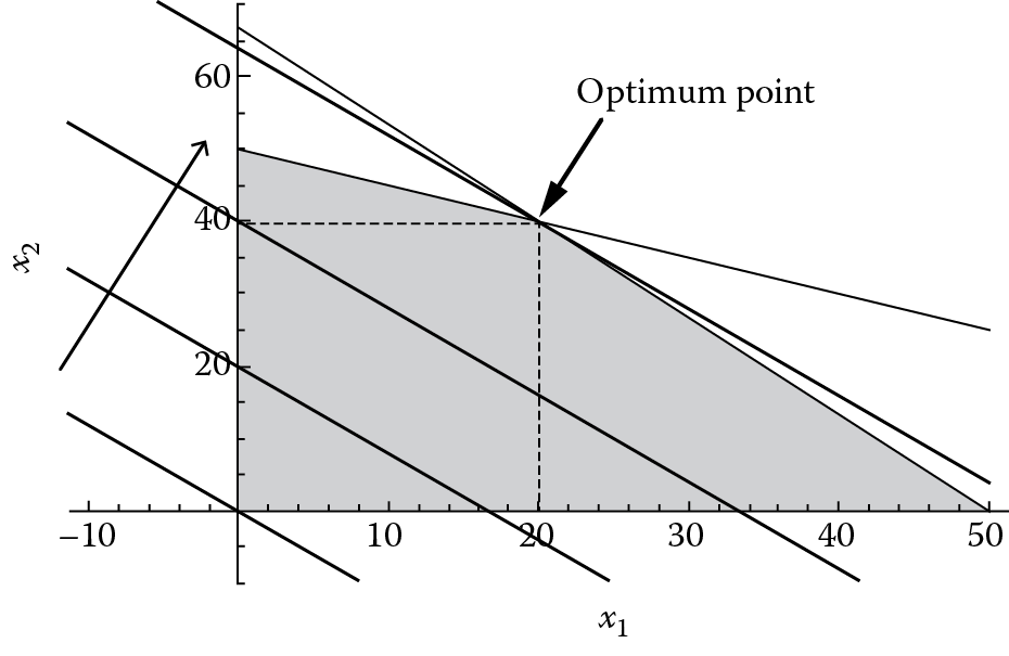
When we move the starting z-line to the right, as indicated by the arrow in Figure 7.8, the value of the objective function increases; we can think of a series of parallel lines with the same slope as x2 = −(6∕5)x1. As long as there are shaded areas untouched by the line, we can still move the line toward the upper right to make the z-value larger, until we arrive at the last point(s) of the feasible region; that is to say, if we move beyond this point, we would leave the feasible region. This means that we have arrived at the maximum value of z, as shown in Figure 7.8. From Figure 7.8 it is easy to see that the optimum point is the intersection point of the two constraint equation lines, x1 = 20, x2 = 40. If we substitute this into the objective function, we can obtain the maximum weekly profit, z = 6(20) + 5(40) = 320 ($). We have to be careful here in identifying the graphical solution, since, sometimes, when we plot the equations, this might not be precise enough for us to obtain the exact answers visually, especially when we are using paper to plot them. We need to vigorously obtain the solution by solving the intersection points of the two constraint equations analytically, that is, solving

$\{\begin{array}{c}4x_1+3x_2=200\\ x_1+2x_2=100\end{array}$

and obtaining the solution x1 = 20, x2 = 40.

From the above example, we can see that usually the optimum points occur at the corner points of the feasible region, assuming that the feasible region is limited and bounded, as in Figure 7.7. However, there are some other possible cases of feasible regions of which readers need to be aware.

7.3.1.2.2 Unlimited Number of Solutions

For the above example, if the objective function becomes z = 8x1 + 6x2, then this objective function is parallel to one of the constraints functions, so ultimately the objective function will not just touch one corner point, but a line segment, that is, the segment P1P2 on Figure 7.9. So every point between P1 and P2 are optimal solutions for the LP model. Since there are an unlimited number of points on the segment, so there are an unlimited number of solutions for this problem.

7.3.1.2.3 Unbounded Feasible Region

If the feasible region is unbounded, as illustrated in Figure 7.10, no matter how far the z-line moves upward, it is possible that the z-line will meet with a corner point. In this case, the optimal solution for this problem is unbounded and does not exist.

The above example illustrates the maximization of an objective function. For the case of minimizing an objective function, we have a similar approach, as follows:

1. Plot all the equations for all the constraints. Similarly to the above example, we first plot the equation for each of the constraints, and then identify the regions that the inequality represents. If we are not sure which side of the equation line the region should be, a simple way to verify this is to take two points, one from each side of the equation line, substitute them into the equation, and see which point satisfies the inequality; then, the region to which that point belongs should be the correct region for that particular constraint.
2. Find the feasible region by identifying the intersection of all the regions of the constraints.
3. Give the objective function a z an initial value, plot the objective function line, then move the objective function parallel to the start line, and toward the direction in which the value of z is reduced (usually to the left and below the axis; first make sure it is touching the feasible region) until the parallel line touches the corner point of the feasible region; this will yield the optimum point for the minimization of the objective function.

   We have prepared some exercise problems at the end of the chapter to both maximize and minimize the objective functions; readers can practice these procedures to see the difference in solving LP maximization and minimization problems. Nevertheless, the graphical method is very simple and intuitive, but the problem is that it only can solve LP models with no more than two (or three, for a 3D plot) control variables. For LP models that involve more than three variables, a general analytical algorithm is needed. The most common algorithm is the Simplex method, which we will discuss in the next section.

7.3.1.3 Simplex Algorithm

The Simplex algorithm requires that the LP problem first needs to be converted to the standard form. From the previous examples, it is easily seen that most of the constraints have the inequality form (i.e., ≤ or ≥). The Simplex algorithm requires that all the constraints are equations, without changing the model; this form of LP is called the standard form of LP. A standard form of LP can described as follows:

$\max z=c_1{x}_1+c_2{x}_2+\cdots +c_n{x}_n={\displaystyle \sum }_{j=1}^n{c}_j{x}_j$

Subject to (s.t.)

$\{\begin{array}{c}{a}_{11}{x}_1+a_{12}{x}_2+\cdots +a_{1n}{x}_n=b_1\\ \\ a_{21}{x}_1+a_{22}{x}_2+\cdots +a_{2n}{x}_n=b_2\\ .\\ .\\ .\\ a_{m1}{x}_1+a_{m2}{x}_2+\cdots +a_{mn}{x}_n=b_m\end{array}{x}_1, x_2, \dots , x_n\ge 0$ (7.20)

Sometimes, we can write the above set of equations as ?? = ?, with

$\mathbb{A}=\left[\begin{array}{cccc}{a}_{11}& a_{12}& \dots & a_{1n}\\ a_{21}& a_{22}& \dots & a_{2n}\\ .& .& & .\\ .& .& & .\\ a_{m1}& a_{m2}& \dots & a_{mn}\end{array}\right]$

and

$x=\left[\begin{array}{c}{x}_1\\ x_2\\ .\\ .\\ .\\ x_n\end{array}\right] , b=\left[\begin{array}{c}{b}_1\\ b_2\\ .\\ .\\ .\\ b_m\end{array}\right]$

There are four characteristics for the standard form of LP:

1. The objective function is a maximization function, max z.
2. All the constraints functions are equations (=).
3. All the decision variables are nonnegative, that is, xj ≥ 0, j = 1, 2, …, n.
4. All the right-hand side constants of the constraint functions are nonnegative, that is, bi ≥ 0, i = 1, 2, …, m.

Based on the definition of the standard form of the LP model, we can easily convert any LP model to a standard form; this is the standardization process of the LP model.

1. Since it is required to maximize the objective function, if the objective happens to be a minimization problem, or $\min z={\displaystyle {\sum }_{j=1}^n{c}_j{x}_j}$ , then we can multiply both sides of the equation by −1 and turn it into a maximization problem; that is to say, the original minimization problem is equivalent to

   $\max z^{\prime }=\min \left(-z\right)=-{\displaystyle \sum }_{j=1}^n{c}_j{x}_j$ (7.21)

2. We need to convert inequalities to equations. Here, we need to use a new concept of slack variables (si ≥ 0, i = 1, 2,…, m), with one slack variable for each constraint.

   If the constraint has the following form,

   ${\displaystyle \sum }_{j=1}^n{a}_{ij}{x}_j\le b_i$

   then we use the slack variable si ≥ 0, so that the constraint becomes

   ${\displaystyle \sum }_{j=1}^n{a}_{ij}{x}_j+s_i=b_i$

   On the other hand, if the constraint has the ≥ form, as follows,

   ${\displaystyle \sum }_{j=1}^n{a}_{ij}{x}_j\ge b_i$

   then we use the slack variable si ≤ 0, to convert the constraint to

   ${\displaystyle \sum }_{j=1}^n{a}_{ij}{x}_j-s_i=b_i$

   By using the slack variables, we can convert inequality constraints to equation forms without changing the constraints themselves.

3. If one of the right-hand side values of a constraint equation is negative, we just need to multiply both sides of the equation by −1 and change its value to nonnegative.

Using the above procedure, we can convert Example 7.2 to the following standard form by adding two slack variables, s1 and s2.

$\text{Maximize}z=6x_1+5x_2$

Subject to (or s.t.)

$4x_1+3x_2+s_1=200\left(\text{assembly constraint}\right)$

$x_1+2x_2+s_2=100\left(\text{painting constraint}\right)$

$x_1,x_2, s_1, s_2\ge 0$

7.3.1.3.1 Concept of LP Solutions

For the LP problem illustrated by Equation 7.20, if X = (x1, x2,…, xn)T satisfies all m constraints, then we call X = (x1, x2,…, xn)T a feasible solution for the LP problem; the set of all feasible solutions is called the feasible set/region of the LP problem.

7.3.1.3.2 Basic and Nonbasic Variables

Consider that ?? = ? has n variables and m linear equations and assume n ≥ m. We can define a basic solution to ?? = ? by setting n − m variables equal to zero and solving the remaining m equations. (Assuming the remaining m variables are linear independent, then according to Cramer’s rule, a unique solution of the m variables exists.)

We call the n − m variables (those equal to zero) nonbasic variables (NBVs) and the solution of the remaining m variables are called basic variables (BVs).

From the above definition, it is easy for us to see that any basic solution in which all variables are nonnegative is a basic feasible solution (BFS). By using the concept of the basic solution, we can easily derive a set of basic solutions for the LP problem initially. We can arbitrarily set n − m variables equal to zero, or if we have m slack variables, we can set all the nonslack variables xj = 0, and make the slack variables si as BVs. The procedure of the Simplex algorithm is an iterative process that substitutes the NBVs with BVs in the direction of increasing the objective function value, yet maintaining the constraints not being violated. It is proven that if the optimal solution for LP exists, then there must exist a basic feasible solution that is optimal. The theorems of optimal basic feasible solutions, and direction and unboundedness, can be found in depth in Winston (1995). In the next section, we will use an example to illustrate how the Simplex algorithm is used to find the optimal solution of LP problems.

7.3.1.3.3 Simplex Algorithm Procedures

The Simplex algorithm consists of five steps to find the optimal solution, described as follows (Winston 1995):

1. Covert the LP to standard form.
2. Obtain an initial basic feasible solution (BFS) from the standard form.
3. Determine if the current BFS is optimal. If yes, then stop. If no, proceed to Step 4.
4. If the current BFS is not optimal, determine which of the NBVs should become a BV, and meanwhile determine which one of the BVs should leave the set of BVs and become an NBV.
5. Use linear equation operations to obtain the value for the new BV and new improved objective value.

Let us use Example 7.2 to illustrate the procedure.

1. Convert the LP to its standard form.

   As illustrated in the previous section, we have converted the LP model to its standard form by using slack variables, as follows:

   $\text{Maximize}z=6x_1+5x_2$

   Subject to (or s.t.)

   $4x_1+3x_2+s_1=200\left(\text{assembly constraint}\right)$

   $x_1+2x_2+s_2=100\left(\text{painting constraint}\right)$

   $x_1,x_2, s_1, s_2\ge 0$

2. Obtain a BFS.

   For this example, the simplest way to obtain a BFS is to let x1 = 0, x2 = 0, and the slack variable can be easily solved as s1 = 200, s2 = 100.

   To perform the iteration of Steps 2, 3, and 4, it is more convenient to use a tabular format to help with the iteration; the table is called a Simplex table, as shown in Figure 7.11.

   Figure 7.11

   

   Simplex table format.

   In Figure 7.11, Columns 2 and 3 (inside the dotted oval area) are the basic feasible solutions (BFSs) and their values (solutions), and those BFSs correspond to the unit matrix in the table, as indicated by the dotted rectangle in the table. The top row is the parameter list of the variables in the objective function, and the left-hand row lists the parameters of the BFSs in the objective functions. When performing the Simplex iteration, only the portion enclosed by the rounded rectangle will perform the linear transformation required; the first two columns change as the BFSs change.

   To illustrate the idea, let us use our example to see how to construct the Simplex table, as shown in Table 7.2.

   Table 7.2

   Initial Setup for Simplex Algorithm for Example 7.2

   c j →			6	5	0	0
   C B	BFS	b	x 1	x 2	s 1	s 2
   0	s 1	200	4	3	1	0
   0	s 2	100	1	2	0	1
   z j			0(4) + 0(1) = 0	0	0	0
   c j − z j			6	5	0	0

3. Test for optimality.

   If all the cj − zj ≤ 0, i = 1, 2,…, n, then we have found the optimal BFSs; stop the iteration and report the results. If there is at least one cj − zj > 0, then a better BFS is possible. If this is the case, move on to step 4. In Table 7.2, at least two cj − zj are positive, 6 and 5. So, we need to find a better BFS.

4. Find a better BFS to increase the objective function value, and update the Simplex table.

   There are three substeps involved in this step; first, we need to find which variable in the BFS set needs to leave the set, and then we need to determine which variable in the non-BFS set needs to enter the BFS set.

   1. Determine the variable to enter the BFS set. One thing we need to mention first is that all the values of cj − zj for all the BFSs are zero (which can be easily seen from the table, since all the BFS correspond to a unit basic matrix, so for each variable in the set of BFS, zj = cj). As mentioned earlier, as long there is one cj − zj > 0, the corresponding xj is eligible to enter the set of BFSs. If there is more than one variable such that cj − zj > 0, we choose the one with the largest cj − zj value; namely, we find k such that

      $c_k-z_k=\underset{j}{\max }(c_j-z_j)$

      From Table 7.2, it is easy to see that x1 should be the variable to enter the set of BFSs, since it has the largest value of cj − zj = 6, so we mark it as Column k, as seen in Figure 7.12.

      Figure 7.12

      

      First step result of the Simplex algorithm.

   2. Determine the variable to leave the set of BFSs. Based on the result from (a), calculate the value of θ for Column k as

      ${\theta }_i=\frac{b_i}{a_{ik}}, i=1,2,\dots , m$

   3. And the row corresponding to the least positive value of θi should be the variable to leave the set of BFSs; namely

      ${\theta }_l=\min \left\{\frac{b_i}{a_{ik}}\text{|}{a}_{ik}>0\right\}=\frac{b_l}{a_{lk}}$

   4. From Figure 7.12, we can easily see that s1 should be the variable to leave the set of BFSs.
   5. Update the Simplex table to obtain a new BFS. First, we need to update Column BFS by replacing s1 with x1, and update the ci column by replacing the corresponding parameter of s1 with that of x1 (changing 0 to 6). A basic row linear transformation is performed in the Simplex table, to change Row k to be part of the basic unit matrix, or to make ${a^{\prime }}_{lk}=1$ (in this case divide the row by 4). To do that, we need to
      1. Divide row l by alk; we have for all the elements in Row l,

         ${b^{\prime }}_l=\frac{b_l}{a_{lk}}$

         ${a^{\prime }}_{ij}=\frac{a_{ij}}{a_{lk}}$ (7.22)

      2. So, from Figure 7.12, we can obtain Table 7.3.
      3. ii. For Column k, transform the element aik = 0, for all aik ≠ alk. Applying the basic linear equation transformation, we have, for all other rows, i ≠ l,

         ${b^{\prime }}_l=b_i-\frac{b_i}{a_{lk}}{a}_{ik}$

         Table 7.3

         Step 1 Iteration Calculation

         c j →			6	5	0	0
         c B	BFS	b	x 1	x 2	s 1	s 2
         6	x 1	200/4 = 50	1	3/4	1/4	0
         0	s 2	100	1	2	0	1
         z j
         c j − z j

         ${a^{\prime }}_{ij}=a_{ij}-\frac{a_{ij}}{a_{lk}}{a}_{ik}$ (7.23)

      4. So, from Table 7.3 we obtain Table 7.4.

Using the procedures in Step 3, we can see that there is one cj − zj > 0, so optimality is not reached yet. Repeat Step 4 to find the variables to enter the set of BFS and leave it; we reach the situation shown in Figure 7.13.

So, we know x2 is the variable entering and s2 is the variable leaving. Applying the basic linear transformation operation from Step 4, we obtain the Simplex shown in Table 7.5.

From Table 7.5, all the cj − zj in the last row have nonpositive values, so the BFS from Table 7.4 with x1 = 20 and x2 = 40 are optimal solutions, and substituting into the objective function we obtain zmax = 6(20) + 5(40) = $320 (Table 7.5).

A comprehensive review of the Simplex algorithm and its extended concepts (including shadow price, duality and sensitivity analysis, and integer programming) are beyond the scope of this text. For a more in-depth review of subject, please refer to any OR text book such as Winston (1995).

7.3.2 Solving LP Using a Spreadsheet

The Simplex algorithm is very straightforward and easy to understand, but it may be tedious, especially when the model size is large; thus, it is suitable to be implemented using computer software. As a matter of fact, there are many scientific computing software packages that include the Simplex algorithm, which makes it easier for us to solve LP models. In this section, we will show how we can use a spreadsheet such as Excel to solve an LP problem.

7.3.2.1 Step 1. Activation of Solver Function in Excel

In Excel, there is an add-in function called Solver that is developed to solve mathematical program models. To use the Solver add-in function, once Excel is open, go to the “File” menu and select “Options”; in the “Excel Options” window, select “Add-Ins”, then in the lower left corner of the “Excel Options” window, choose “Excel Add-Ins” and click the “Go…” button, as shown in Figure 7.14.

Once the “Go…” button is clicked, the dialog window shown in Figure 7.12 will pop up; check the option of “Solver Add-in” and then click on “OK”, as shown in Figure 7.15.

Once the “Solver Add-in” option is selected, go back to the Excel main menu, and select the “Data” tab; you will notice that a new analysis button has been added at the upper right of the menu bar, as shown in Figure 7.16.

We will be using this function to solve the LP problem. But, before that, we need to set up (formulate) the LP model properly in Excel.

7.3.2.2 Step 2. Set-Up of LP Model in Excel

Let us use Example 7.2 to illustrate how to set up the LP model. Open a new worksheet, select an area for control variables and use these variables to express the objective function, as shown in Figure 7.17.

In another area (usually below the control variables), set up the constraints, as shown in Figure 7.18.

In cells E6 and E7, we need to insert the formula on the left-hand side of the constraint inequality, as shown in Figure 7.19.

7.3.2.3 Step 3. Solving the LP Model

Once the model has been properly set up, click on “Solver” on the “Data” tab, click the button on the right and select the right cells, as indicated in Figure 7.20.

Next, click on the “Add” button, adding the constraints, again by using the button and select the appropriate cells from the worksheet, choose the “select a Solving Method” as “Simplex LP”; after all these are complete, click the “Solve” button (Figure 7.21). The results of the control variables and objective values will be updated in the worksheet, as shown in Figure 7.22.

From the results, x1 = 20 and x2 = 40, the maximum objective value z = $320.

7.4 Summary

Systems engineering makes efficient use of resources to develop complex system functions, since most resources are limited and scarce. Optimizing the utilization of these limited resources has always been a challenge for system designers. Optimization can be defined as a procedure/algorithm to determine the value of independent (or control) variables to maximize (or minimize) the value of objective functions. In this chapter, we reviewed some of the most common used models in systems engineering practice. First, we introduced the concepts of unconstrained optimization models. These models are based on basic differentiation theory. If a function f(x) is differentiable, then the local optimum can be obtained by Fermat’s theorem; that is to say, the first-order derivative of f equals zero. Fermat’s theorem only gives a necessary condition for finding the local optimum; it only shows if a point is a reflection point. To confirm that the reflection is truly a local maximum (or minimum) point, a higher order of differentiation is needed. If the second-order derivative is negative, then the point is a local maximum; if the second-order derivative is positive, then the point is a local minimum.

In the second part of the chapter, we described constrained optimization models using mathematical programming. The fundamental form of mathematical programming is LP. With LP models, both the objective functions and constraint functions are linear. LP models are formally defined and we used some examples to illustrate how to formulate a LP model. If an LP model has only two or three decision variables, we can solve it by using graphical methods. If more than three variables are involved, we need to apply a more general algorithm called the Simplex method. A tabular format of the Simplex algorithm was described in detail, and at the end of the chapter, we briefly discussed how to use spreadsheet software to implement the Simplex method.

Optimization plays an important role in the system engineering design process. This chapter provides a basic review of the most commonly used optimization models for systems engineers to understand the nature of optimization problems. For a more in-depth review of these materials, it is recommended to look at an OR text as mentioned in the chapter.

Problems

5. Define optimization. Why is optimization important in systems engineering?
6. If $f\left(x\right)=\ln \sqrt{1+x^2}$ , what is f′(0)?
7. If f(x) = xn + 2e, find f(n)(x).
8. If x ∈ ℝ, what is the reflection point for function y = f(x) = 3x3 − 27x? Is this point a minimum point or maximum point? Why?
9. Using unconstrained conditions, find the minimum point for the function f(x1, x2)

   $f\left(x_1, x_2\right)={\left(x_1^2-1\right)}^2+x_1^2+2x_2^2-2x_1)$

10. The cost of a product A is C(x) = 16x + 250 (thousand dollars), with x being the number of items produced; the total revenue after selling all the x products is R(x) = 24x − 0.008x2 (thousand dollars). What should x be to maximize the total profit (revenue-cost), and what is the maximum profit?
11. Formulate the following using an LP model:

    A company makes two types of toy product, Product A and Product B. Product A makes $50 profit/unit, and Product B makes $40 profit/unit. There are four work stations that are needed to produce A and B; Product A uses Stations 1, 2 and 3 and Product B uses Stations 2, 3, and 4. The hours needed for the two products are listed in the following table as well as the daily production capacity for each of the stations (in hours). Make a daily production plan for this company to maximize the profit (Table 7.6).

    Table 7.6

    Station	Product A Requirement (h)	Product B Requirement (h)	Daily Capacity (h)
    1	2	0	300
    2	0	3	540
    3	2	2	480
    4	1	2	300

12. A small furniture company makes four different types of furniture, using wood and glass as the materials. The production requirements and daily capacity for labor hours and materials are listed in the following table. Formulate it using LP (Table 7.7).
13. Solve the following LP problems graphically.
    1. max z = 2x1 + 3x2

       $\text{s}\text{.t}\text{.} \{\begin{array}{l}{x}_1+x_2\le 4\hfill \\ 4x_1\text{+3}{x}_2\le 16\hfill \\ 4x_2\le 12\hfill \\ x_1,x_2\ge 0\hfill \end{array}$

       Table 7.7

       Furniture Type	Labor Hours Needed (h/unit)	Wood (per unit)	Glass (per unit)	Profit ($/unit)	Maximum Allowable Production (units/day)
       1	2	4	6	60	100
       2	1	2	2	20	200
       3	3	1	1	40	50
       4	2	2	2	30	100
       Daily capacity	400	600	100

    2. max z = x1 + 3x2

       $\text{s}\text{.t}\text{. }\{\begin{array}{l}6x_1+7x_2\le 50\hfill \\ x_1 \ge 3\hfill \\ x_2\ge 2\hfill \\ x_1,x_2\ge 0\hfill \end{array}$

    3. min z = 6x1 + 4x2

$\text{s}\text{.t}\text{.} \{\begin{array}{l}2x_1+x_2\ge 1\hfill \\ 3x_1+4x_2\ge 3\hfill \\ \hfill \\ x_1,x_2\ge 0\hfill \end{array}$

14. Solve the above LP problems using a spreadsheet.
15. Solve Problem 6 (the one associated with Table 7.6) using Excel. Is it economically feasible for the company to pay $10 for an employee to work one extra hour every day?