CHAPTER
7
Content distribution networks
From the invention of telegraph and the start of electrical communications, distribution channel technology has governed the amount of information that could be transmitted in a given time interval. No matter how one tries, the physics of the distribution channel determine how much information can fit in the pipe.
Bandwidth is a fundamental characteristic of a communications channel. It is a measure of data transfer capacity. Bits per second metrics are used for serial, single-wire paths; bytes per second metrics are used for parallel data transfers; and symbols per second metrics are used for more sophisticated methods of digital transmission.
Content distribution networks can be broken down into two primary categories: consumer and commercial. Consumers are end users receiving content wirelessly over the air and over a wired physical distribution technology. Each method has its pros and cons as well as implementation suitability scenarios. Content distribution to consumers will be covered in Book 2.
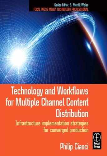
Content producers and broadcasters use sophisticated distribution networks that ensure maintenance of the highest possible audio and video quality. Professional content delivery networks are used in three phases of the content life cycle.
During content creation, electronic newsgathering (ENG) trucks or remote venues feed content back to an operations center. This backhaul acquisition of content is assembled into a format for distribution. However, disseminating the content can be done in a number of ways.
If the production and transmission site are colocated, signals can be released over the distribution channel. This is rarely the case. Consider a radio broadcaster located in a city. The program originates from a studio location, but the transmitter is in the suburbs. The program must now be sent to the transmitter over a studio transmitter link (STL) that uses technology that is incompatible with consumer reception.
Similarly, a TV network releases programming to affiliates over dedicated commercial transmission paths. Local commercials are inserted at each of the affiliate stations. When sending an e-mail, the signal on the cable to your computer hits the ISP gateway and traverses over the Internet's commercial backbone until it reaches a mail server on a network that can be accessed by the recipient. There the message is downloaded over a dedicated connection to the recipient's computer.
Before delving into content production, an understanding of the technology and limitations of each channel will explain constraints on creating and assembling content for each delivery method and consumer platform.
DISTRIBUTION SCENARIOS
Transporting broadcast quality digital content presents unprecedented challenges. With analog signals noise, signal strength and reflections were of paramount concern. Channel bandwidth only needed to support baseband signals: 6 MHz for NTSC system and 8 MHz for PAL and SECAM.
Compressed video and audio requires attention to a new set of technical issues. Since compression is usually lossy and perceptual based, as the bit rate is reduced, increasingly more high-frequency information is lost. As low bit-rate content travels through the production workflow, additional decompression/compression cycles will discard more information. Eventually, audible and visible artifacts will be perceived.
To mitigate the loss of information, higher bit-rate audio and video formats are used in transferring content to, from, and between broadcast sites and operations centers. Low bit rates, 19.39 Mbps for ATSC DTV, are used only for finished content meant for consumer distribution.
Backhaul and contribution feeds from remote venues use bit rates from 38 Mbps up to 220 Mbps for HD and 40 Mbps for SD video content. Distribution for network release may use a mezzanine level of compression, typically 45 Mbps. The data rate is dependent on the delivery channel, and cannot exceed the lowest bandwidth anywhere on the transmission path.
An STL is used to transfer finished programs to the transmission site; a 19.39 Mbps MPEG-2 transport stream over an ASI or SMPTE 310 interface is sufficient.
Figure 7.1 illustrates how content is distributed to and from segments of the broadcast chain.
Terms describing different areas of content distribution tend to be used loosely. Contribution and backhaul are sometimes used interchangeably; so are distribution, release, and mezzanine.
This chapter will discuss the technology used to backhaul, contribute, and distribute high bit-rate content between operation centers, transmission site, and consumer distribution nodes.
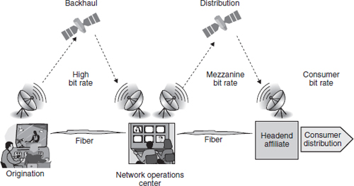
FIGURE 7.1
Distribution technology interdependence during the content life cycle
THE ORIGINS OF TELEVISION LONG-HAUL DISTRIBUTION
AT&T demonstrated long-distance transmission of television in 1927. An experimental electromechanical system scanned 50 lines of resolution at 16 times per second and transmitted the signal over telephone lines from Washington, DC to Whippany, NJ, and then over a radio link to New York. This established the long-haul paradigm that was to remain in place for TV signal long haul until the 1970s: a combination of RF and cable technologies.
Researchers at Bell Labs patented coaxial cable in 1929. Although developed to increase telephone transmission capacity, it turned out to be well suited for long-distance TV transmission. It had an astounding bandwidth for its time—1 MHz, which was a great improvement over unshielded cabling bandwidth. By 1936, experimental coaxial cable was run between New York and Philadelphia, with signal booster stations every 10 miles (16 km).
After this experiment, AT&T discontinued work on electromechanical television, and as conventional industry intelligence realized, the future of TV would be an all-electronic system. Prototype systems were invented and constructed independently by Vladimir Zworykin and Philo T. Farnsworth. The first electronic television system to go on the air was the 405-line UK system in 1936 developed by John Logie Baird.
Bell Labs gave demonstrations of the New York–Philadelphia television link in 1940–1941. AT&T used the coaxial link to transmit the Republican National Convention in June 1940 from Philadelphia to New York City, where it was televised to a few hundred receivers over the NBC station.
NBC had earlier demonstrated an intercity television broadcast on February 1, 1940, from its station in New York City to WRGB in Schenectady, NY using General Electric relay antennas, and began transmitting some programs on an irregular basis to Philadelphia and Schenectady in 1941. Wartime priorities suspended the manufacture of television and radio equipment for civilian use from April 1, 1942 to October 1, 1945.
In 1946, AT&T completed a 225-mile (362 km) cable between New York City and Washington, DC. The DuMont Television Network, which had begun experimental broadcasts before the war, launched what Newsweek called “the country's first permanent commercial television network” that same year, connecting New York with Washington, DC. Not to be outdone, NBC launched what it called “the world's first regularly operating television network” on June 27, 1947, serving New York, Philadelphia, Schenectady, and Washington, DC.
In the 1940s, the term “chain broadcasting” was used, as the stations were linked together in long chains along the east coast. But as the networks expanded west-ward, the interconnected stations formed networks of connected affiliate stations.
When television broadcasting began in earnest after the conclusion of WWII, AT&T began providing transmission for broadcasters over cable between Washington, DC., and New York. The initial distribution network was expanded by the addition of a microwave-relay transmission system between New York and Boston in 1947. When it was connected to the New York–Washington cable, television networking from Boston to Washington, DC was possible.
In 1951, AT&T completed the construction of their microwave radio relay network of AT&T Long Lines, the first transcontinental broadband-communications network, and carried all four existing TV networks coast to coast. President Harry Truman's September 4 address to the United Nations/Japan Peace Treaty Conference is the first live transcontinental television broadcast.
These networks were the only way to distribute TV programs nationally until two technologies developed in the 1960s and commercialized in the 1970s revolutionized long-haul television distribution: satellites and fiber optics.
DISTRIBUTION TECHNOLOGIES
Distribution technology can be divided into two categories: those that are freely propagated over a medium and those that are carried over some kind of physical conveyance. Radio frequency transmission is an example of the former, while cable-based transmission is an example of the latter.
RF transmission is over the air, or via satellite. Cable infrastructures are either wire-based or optical. There is one exception: for high power, RF wave guides are used, but these are beyond the scope of this discussion.
Radio wave propagation in space
Radio waves are electromagnetic waves that propagate through space. There are three types of radio waves: ground, space, and sky. Figure 7.2 illustrates the different transmission characteristics of each type.
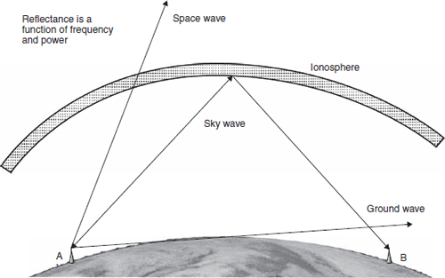
FIGURE 7.2
Radio wave propagation through free space
Consider what happens for each type of wave when transmitted from point A. A ground wave is eradiated in all directions from the transmitter. A ground wave will not be received at station B because of the curvature of the earth. A space wave travels through the ionosphere and is usually a concentrated, directional beam. Sky waves bounce off the ionosphere and return to earth over a greater distance than ground waves. In this example, they are the only type of the three that can facilitate communication between point A and point B.
Microwave
Microwave transmission refers to the technique of transmitting information over a microwave link. Microwaves are electromagnetic waves with wavelengths shorter than one meter and longer than one millimeter, or frequencies between 300 MHz and 300 GHz. Due to the fact that signals in this frequency range are affected by rain, vapor, dust, snow, cloud, mist, and fog, the successful implementation of microwaves is generally limited to line-of-sight transmission links without obstacles.
Because a line-of-sight radio link is made, the radio frequencies used occupy only a narrow path between stations. Antennas used must be highly directional; these antennas are installed in elevated locations such as large radio towers in order to be able to transmit across long distances.
Typical types of antenna used in radio relay link installations are parabolic reflectors, shell antennas, and horn radiators, which have a diameter of up to four meters. Highly directive antennas permit an economical use of the available frequency spectrum, despite long transmission distances.
Satellite
Placing an artificial moon in orbit around the Earth had long been a dream of many a scientist. Isaac Newton first revealed the physics and mathematical principles required to do it, although it could not be accomplished until more than two centuries after his death.
Arthur C. Clarke described the concept of a stationary orbiting object in October 1945 in a paper titled Extra-Terrestrial Relays—Can Rocket Stations Give Worldwide Radio Coverage?, published in Wireless World. The geostationary orbit is a special case that occurs when a satellite's angular velocity matches the Earth's. The object in orbit will remain in a fixed position relative to the surface of the Earth.
In 1957, the Soviet Union launched Sputnik. While the world was in awe, the U.S. industrial–military complex was in shock. Military leaders understood the strategic importance surveillance and communication orbiting satellites would have, especially with further development and refinement. In addition, the ability to deliver a nuclear weapon via intercontinental ballistic missile (ICBM) was closer to fact than to fantasy during the Cold War. The United States had to be in space.
Launch failures by the United States were forgotten when Explorer I made it to orbit in January 1958. While Sputnik simply transmitted a periodic radio beep (at a frequency that could be picked up by ham radio operators) back to the Earth, Explorer was packed with scientific instruments. When the telemetry transmitted back to the Earth was deciphered, radiation belts around the Earth were discovered and named after James Van Allen, a professor at Ohio State who designed the on-board instruments for the Jet Propulsion Laboratory.
Communication via space
In the 1950s, J. R. Pierce and his associates at Bell Labs began work on satellite communications concepts. At that time the responsibility for all communications satellites rested with the military.
The National Aeronautics and Space Administration (NASA) was established in July 1958, by the National Aeronautics and Space Act. Two years later, Congress defined the scope of civilian and military space efforts: NASA would conduct research with “mirrors” or “passive” communications satellites, while synchronous and “repeater” or “active” (satellites that amplify the received signal at the satellite) satellites would be a Department of Defense effort.
Echo 1A, a metallic balloon, was placed in low Earth orbit (LEO) by a Delta launch vehicle in August 1960. The first communications satellite “Echo” could be seen with the naked eye.
In 1960, AT&T filed with the Federal Communications Commission (FCC) for permission to launch an experimental communications satellite. By the fall of 1960, AT&T began development of a satellite communications system called Telstar. The operational system would consist of “between 50 and 120 simple active satellites in orbits about 7,000 miles high.”
The Influence of the Space Program on Digital Technology
Soviet rockets could carry a considerably heavier payload than U.S. rockets. Due to this “missile gap,” great importance was placed on the need to miniaturize electronic systems. As a national defense priority, refinement of integrated circuit (IC) fabrication progressed rapidly. At one point in the 1960s, it is said that 60% of all the ICs produced were for the space program. The missile gap disappeared with the development of the F1 engine and the Saturn moon rockets.
It's difficult to hit a moving target
A satellite in orbit travels at over 17,800 mph; therefore, the amount of time in which a signal can be sent from point A to point B over a satellite link is limited to minutes. This is why Bell Labs envisions a network of orbiting communications satellites. Using cellular concepts, signals would be handed off to a trailing satellite when the satellite currently broadcasting the signal moved out of range of the ground stations.
A better solution was needed if the use of space for dependable communication had to be viable and commercially profitable.
Deployment accelerates
Bell Telephone Laboratories continued its pioneering work and designed and built the Telstar spacecraft. The first Telstars were prototypes that would prove the concepts behind the constellation system that was being planned. NASA's contribution to the project was to launch the satellites and provide some tracking and telemetry functions, but AT&T bore all the costs of the project, reimbursing NASA $6 million.
Telstar I was launched on July 10, 1962, and once in orbit, it immediately broadcast live television pictures of a flag outside its ground station in Andover to France. The first “official” transmissions occurred on July 23, when a short segment of a televised major league baseball game between the Philadelphia Phillies and the Chicago Cubs at Wrigley Field was transmitted to Pleumeur-Bodou, France. On that day the first satellite telephone call, faxes, and data transmissions were also performed.
The first geosynchronous communication satellite, Syncom 2, was launched in 1963, and by 1964, two Telstars, two Relays, and two Syncoms were operating successfully in space. During this time, the Communications Satellite Corporation (COMSAT), formed as a result of the Communications Satellite Act of 1962, was contracting for their first satellite. COMSAT ultimately chose geosynchronous satellites proposed by Hughes Aircraft Company for their first two systems and TRW for the third. On April 6, 1965, COMSAT's first satellite, also the world's first commercial communication satellite, Intelsat I (also called Early Bird), was launched from Cape Canaveral.
FIGURE 7.3
Low, medium, and geostationary orbits
Satellites can be deployed at various altitudes above the Earth: LEO, medium Earth orbits (MEO), and geosynchronous orbits, which have become the de facto orbit for communication satellites. Figure 7.3 compares orbital types.
Today satellites are an integral component of content and data distribution. However, rather than remaining strictly divided, satellite, cable, and terrestrial transmission together form content distribution networks.
Superstations pave the way
Cable TV systems were little more than local aberrations in the broadcast universe until satellites were brought into the picture. In the late 1970s, Ted Turner had the idea of distributing WTCG in Atlanta via C-band to cable systems across the United States. Now available across the country, WTCG (later changed to WTBS and now WPCH) became the first “superstation.”
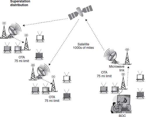
FIGURE 7.4
Superstation national television distribution
Turner's distribution method changed the rules of the game. FCC Rules and Regulations in 47 CFR 77.120 define a “nationally distributed superstation.” The general requirement is that the station is “not owned or operated by or affiliated with a television network,” offers “interconnected program service on a regular basis for 15 or more hours per week to at least 25 affiliated television licensees in 10 or more states,” and is retransmitted by a satellite carrier. Figure 7.4 illustrates the long-distance distribution technique.
The significance of this conceptual innovation was that when Cable News Network, CNN, was launched in 1981, Turner used the same national content distribution paradigm: satellite uplink and national distribution via downlink to cable headends. So, in a very real sense, superstations morphed into national cable TV broadcasting systems.
AT&T innovates
AT&T launched its first Telstar III domestic communications satellite in 1983. This resulted in a short-lived attempt to introduce direct-to-home satellite broadcasting. Japanese television had already implemented such a system and planned to use it to deliver its MUSE HDTV system.
AT&T continued to expand its commercial television contribution and distribution network. Optical networks and satellite systems were integrated. Its Littleton, CO-based operations center, Headend in the Sky (HITS), became a major distributor of content to MSOs, delivering more than 170 digitally compressed video and audio TV programming signals to 3,000-plus cable operation sites across the United States. AT&T got out of the satellite business in 1994 when it sold the fleet to Loral. In 2001, Comcast acquired AT&T Broadband, HITS, and AT&T's cable TV business.
Satellite transmission technology
Satellite television systems consist of Earth and space segments. The transmitting antenna is located at an uplink facility. Uplink satellite dishes are very large, as much as 9–12 meters (30–40 feet) in diameter. Transmission is in the C-band or Ku-band or both. A high band, the Ka-band, is being increasingly utilized. Table 7.1 lists the uplink and downlink frequencies for each band.
An uplink dish is pointed toward a specific satellite, and the uplinked signals are transmitted within a particular frequency in a band and are received by one of the transponders tuned to that frequency aboard that satellite.
The transponder “retransmits” the signals back to the Earth at a different frequency band (a process known as translation that is used to avoid interference with the uplink signal). The leg of the signal path from the satellite to the receiving Earth station is called the downlink.
Satellites have up to 32 transponders for Ku-band or 24 for a C-band. Typical transponders each have a bandwidth between 27 MHz and 50 MHz. C-band transmission is susceptible to terrestrial interference, while Ku-band transmission is affected by atmospheric moisture.
Each geostationary C-band satellite needs to be spaced 2° from the next satellite to avoid interference. For Ku the spacing can be 1°. This places a limit on the total number of geostationary C-band and Ku-band satellites at 180 and 360, respectively.
The power of a radio transmission decreases in proportion to the square of the distance it travels. A weak downlinked signal is reflected by a parabolic receiving dish to a feedhorn at the dish's focal point. This feedhorn is the flared front end of a section of waveguide that “conducts” signals to a probe or pickup connected to a low-noise block (LNB) downconverter. The LNB amplifies the weak signals, filters the block of frequencies in which the satellite TV signals are transmitted, and converts the block of frequencies to a lower frequency range in the L-band range, 950–1450 MHz.
Table 7.1 Satellite Frequency Bands |
||
Frequency band |
Downlink |
Uplink |
C |
3,700–4,200 MHz |
5,295–6,425 MHz |
Ku |
11.7–12.2 GHz |
14.0–14.5 GHz |
Ka |
17.1–21.2 GHz |
27.5–31.0 GHz |
The satellite receiver demodulates and converts the signals to television, audio, or data. If the receiver includes the capability to unscramble or decrypt, it is called an integrated receiver/decoder (IRD). The cable connecting the receiver to the LNBF or LNB should be of low loss type, such as RG-6 or RG-11.
Fiber-optic communication
Fiber-optic systems consist of a light transmitter (laser or LED); an optical medium (glass or composite); and a photodetector receiver.
The first prototype laser (an acronym for Light Amplification by Stimulated Emission of Radiation), was a synthetic ruby crystal device demonstrated in 1960 by Hughes Research Laboratories. Although commercial lasers became available in 1968, it took refinements to glass purity by Corning and the development of room-temperature operational semiconductor diode lasers at Bell Labs in the early 1970s to make fiber optics a viable commercial technology.
A variety of light-emitting technologies are used in transmitters. Fabry-Perot lasers or distributed feedback (DFB) lasers are used in long haul and high data rate applications. Vertical-cavity surface-emitting lasers (VCSELs) are suitable for shorter-range applications such as Gigabit Ethernet (GigE) and Fibre Channel. Light-emitting diodes (LEDs) are used for short-to-moderate transmission distances. LEDs are the least-expensive transmitters but have limited data capacity.
Figure 7.5 shows the development of, and subsequent improvement in, fiber-optic wavelength windows over the last few decades. Appropriate transmitter technology is also indicated for each window.
Two types of photodetectors, avalanche photodiode (APD) and positive-intrinsicnegative (PIN), convert photons of light to electrons. Because of the small number of photons received, amplification is necessary to recover data and produce a usable signal. APD amplification is internal, while the amplification is external for PIN detectors.
Fiber-optic systems use a variety of signal multiplexing techniques. Time-division multiplex (TDM) assigns data packets to time slots and is used in long-haul infra-structures. Wave-division multiplex (WDM) enables multiple wavelengths of light to share a single fiber. In first-generation deployments, WDM technology supported just two wavelengths, also referred to as “lambdas,” usually 1,310 and 1,550 nm.
As fiber-optic technologies improved, it became possible to transmit more than two lambdas simultaneously over a single fiber strand. This resulted in the development of coarse wave-division multiplex (CWDM) and dense wave-division multiplex (DWDM). DWDM uses narrow channel spacing, frequently 0.8 or 1.6 nm, while CWDM spaces channels 20 nm apart. Figure 7.6 illustrates implementation of each technique as specified in ITU-T standards.
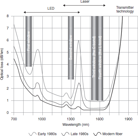
FIGURE 7.5
Improvements in fiber optics
Single-mode fiber (SMF) carries a single wavelength of light and is suited for long runs, such as between buildings, venues, and broadcast sites (STL, TSL, intracity, and intercity links), for long camera runs and as risers in facilities. SMF cables are yellow. Fiber cores are 8.5 micrometers in diameter. Something of an oxymoron, SMF is best suited for DWDM implementations. This is because DWDMs pack multiple lambdas so tightly that the bundle can be transmitted as a “virtual single” wavelength.
Multimode fiber (MMF) can carry multiple wavelengths on a single strand. They are used in short runs generally inside a building and are identified by their orange color.
SMF technology is more expensive to implement than multimode. Lasers must be precisely tuned, and cannot use the less expensive LEDs transmitters found in CWDM links.
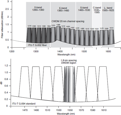
FIGURE 7.6
Comparison of CWDM and DWDM
DIGITAL SIGNALING
Analog television transmission has all but completely disappeared. Digital rules! Digital transmission is enabled by audio and video compression technology. HD data rates of 1.5Gbps require a 50:1 data reduction to enable them to be carried in a 6MHz channel.
Digital transmission and reception is an all-or-nothing proposition. Either the signal can be perfectly decoded or virtually not at all. This characteristic is called the cliff effect.
Decoding accuracy rapidly deteriorates in the cliff area: “salt and pepper”, macro-blocking, and other artifacts become perceptible. Error correction and concealment techniques are implemented to extend the ability of receivers to recover and decode corrupted digital signals.
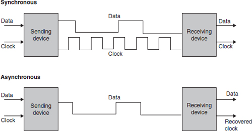
FIGURE 7.7
Synchronous and asynchronous data transmission
Random, constant, and deterministic
Digital data transfers can be broken down into three categories. The first is synchronous, where data is continuous at a given, uninterrupted rate over time. SDI is a synchronous digital signal.
Asynchronous data transfer techniques can be illustrated by the Internet; packet delivery has no fixed relationship to time. A download can be virtually instant, or can crawl at peak usage times. The packet transfers, and subsequently the number of data bits, have no fixed relationship to a constant duration of time. This is bad for both real-time delivery and media presentation.
Synchronous data transfers, as shown in Figure 7.7, are enabled by transmission of the data along with a clock signal. The receiver uses the clock to identify when data is valid. In an asynchronous system, data is encoded in such a way that the receiver can recover the clock signal and then interpret the information present in the signal to recover the data.
Isochronous data transfer is a technique that delivers a defined quantity of bursty data in a given time duration is called (Figure 7.8). In this way, a device can expect a certain amount of data and needs only to be able to buffer within specified maximum and minimum amounts.
Reception of bursty data can be a problem. Processing circuits and algorithms, especially real-time systems, expect data to be available on a continuous basis. Techniques have been developed to supply data when needed.
Buffering: smoothing out data bursts
In order for a digital processing devices to operate in real time, a defined amount of data must be transferred over a given time period. Buffering is a technique that smooths out bursty data received over a transmission channel.
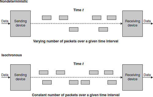
FIGURE 7.8
Isochronous communication transmits a constant number of packets over a defined time interval
In order for a buffer to perform its function properly, data must be isochronous. Isochronous data transfers supply a defined amount of data in a given time period, with no specification of maximum or minimum burst size. This specification enables the design of buffers with adequate memory allocation.
A smoothing buffer accepts bursts of data packets and stores them in RAM. This enables access by processing devices at a predictable data rate.
Consider the scenario where a device requires a constant data rate of 100 Mbps and data can burst at 200 and 50 Mbps. As shown in Figure 7.9, data is initially written into a buffer at 100 Mbps for two seconds. Data readout is delayed until after one second when the buffer holds 100 Mb of data. Next, two seconds of 200 Mbps data is fed into the buffer, and at the three-second mark, 300 Mb remain in the buffer (400 Mb have been written into the buffer, while 200 Mb have been read out; add the original 100 Mb and 300 Mb are left in the buffer). The variable data rates are well behaved and can be accommodated as shown.
A buffer smooths variable data rates, enabling a 100 Mbps readout.
If too much data arrives in a given time period, the buffer will overflow and packets will be lost. Figure 7.10a illustrates this situation. The buffer can hold 400 Mb of unread (or unprocessed) data. As in Figure 7.10b, data arrives at 100 Mbps for the first two seconds. After the first second, data readout begins. The data rate now increases to 200 Mbps, and after three more seconds, the buffer is full. During the next second, half of the data that arrives at 200 Mbps is stored and read out, and the other half is lost. If the data rate now falls to 50 Mbps, data can be read out again at 100 Mbps. After two seconds, in this example, the data rate returns to 100 Mbps and the buffer stabilizes with 300 Mb of its capacity used.
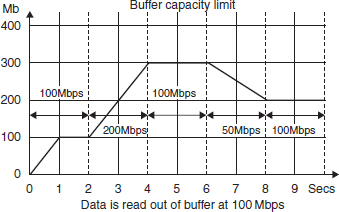
FIGURE 7.9
Buffer fullness as a function of data rate
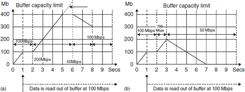
FIGURE 7.10
Buffer overflow and underflow conditions. In (a, left), a buffer overflows and loses data when data arrival exceeds the buffer capacity. In (b, right), a buffer underflows and data is not available for processing when it is read out at 100 Mbps
Figure 7.10b follows the same pattern for the initial three seconds as described in Figures 7.10a. After three seconds, the buffer has 200 Mb of data stored. Data now arrives at 50 Mbps, and after four seconds of reading out data at 100 Mbps, the buffer is empty. As data continues to arrive at 50 Mbps, the buffer cannot supply sufficient data to support a 100 Mbps readout.
In the underflow condition, a processing device will be starved for data. This makes real-time device performance (processing) impossible. Conversely, in the overflow condition, the processing device will have too much data to process; hence, it will choke. Real-time processing will continue but with lowered quality, because data will be lost.
BACKHAUL AND CONTRIBUTION
Transporting remotely originating program content back to the studio is referred to as backhaul. Broadcast auxiliary service (BAS) was an early method that got the job done. BAS is still in use today.
Two methods are generally in use for remote broadcasts. One places a production control room, often a truck, at event sites and backhauls produced content back to the operations center for commercial, logo, closed caption, and other content and overlay insertion. The other is an emergent technique that backhauls individual elements to the operations center where audio and video sources, along with graphics, are assembled in a PCR.
Virtually 100% of all TV programming is distributed in a compressed digital form. Each method of transfer has particular technology and content formats associated with it.
Because of the limited distances radio waves can propagate, from the earliest days of radio, programming was distributed using cables over long distances to broadcast operation centers for over-the-air transmission.
Today, because of the data rate demands of contribution-quality HD, content distribution systems require an upgrade to 270 Mbps or greater. Some HD IP video backhaul solutions are based upon JPEG2000 compression, a wavelet technology that enables frame-accurate processing. Using JPEG2000 compression, the bit rate of 1.485 Gbps for HD-SDI can be reduced to between 50 Mbps and 200 Mbps; rates then can be carried over an OC-3 or OC-12 network, respectively.
JPEG2000 is wavelet-based and encodes each frame independently. It provides 10-bit resolution inherent in the HD-SDI format. HD television formats supported are 720p59.94, 1080i59.94, 720p50, and 1080i50. JPEG2000 has been selected as the standard file format for digital cinema. It does not create blocking defects and support resolutions beyond 10-bit HD.
Broadcast auxiliary service
In the early days of broadcasting, production and transmission operations were often in the same location. Content was distributed from the studio to production control rooms over the facility routing infrastructure. This consisted of cables and patchbays, much like existing telephone switchboards. Connecting signals between master control and the transmitter could be accomplished using cabling.
However, as the need to transport signals from locations outside of the operations center increased, BAS was developed. Microwave links were frequently used. Figure 7.11 shows the various BAS scenarios.
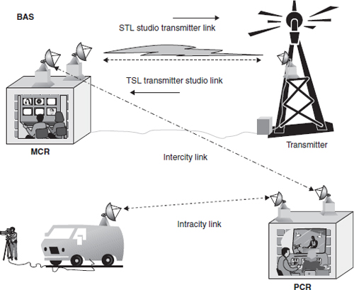
FIGURE 7.11
Studio-transmitter, transmitter-studio, intracity, and intracity links
A microwave BAS link is a simplex or duplex communication circuit between two points utilizing a single frequency/polarization assignment. A duplex communications circuit would require two links, one link in each direction.
BAS frequency bands include 450 MHz, 2 GHz, 7 GHz, 13 GHz, 40 GHz, and the entire broadcast TV spectrum. IFB and two-way microphone communications use the 450 MHz band. The other bands are used for ENG intercity relay (IRC) and in either direction between the studio and the transmitter (STL/TSL).
BAS, is defined in 47 CFR, Parts 101 and 74.
Electronic newsgathering
Coverage of breaking stories is a staple of news broadcasts. Every station in a local market is striving to break a story first or get that one crucial, newsworthy shot on air. BAS transmissions are often used to get the content back to the broadcast center. Usually referred to simply as ENG, electronic newsgathering is a representative example of the transmission chain used by BAS. Figure 7.12 represents the functional blocks of the transmission and receiving equipment.
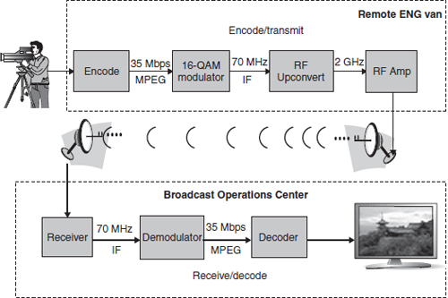
FIGURE 7.12
ENG microwave functional diagram
In this example, the content acquired by the camera operator in the field is compressed using MPEG-2 to a 35 Mbps data rate. This is a high enough rate to allow editing and maintain image quality. 16-QAM modulation produces a 70 MHz intermediate frequency, which is upconverted to a 2 GHz signal for transmission. The dishes are in a line of sight, and at the broadcast operations center, the signal processing is reversed, and the audio and video are ready for editing or live broadcast.
2-GHz BAS relocation
The 2 GHz frequency range is a BAS band primarily used for ENG. Nextel cellular services utilized frequencies in the 800 MHz spectrum range. Unfortunately, this band was also used by public safety licensees. The result was unwanted interference. The FCC solution, reached in 2004, was that Nextel would relinquish its 800 MHz spectrum in return for new allocations in the 2 GHz range. In exchange, Nextel would underwrite the movement of all BAS services. This is known as the 2-GHz BAS relocation plan.
The relocation requires the conversion of each 2 GHz system to a new FCC-mandated frequency allocation and channel plan. This consists of seven digital channels operating at 2,025–2,110 MHz. The new frequency allocation reduced channel widths from 17 MHz to 12 MHz and required digital COFDM transmission. For the first time, the FCC has forbidden analog transmission in a BAS frequency band.
As part of the terms of the relocation agreement, Nextel is required to provide “comparable facilities” to eligible broadcasters for digital operation in the new, reduced bandwidth channel plan. This requires that the existing 2 GHz transmitters, receivers, central receive antennas, and remote controls be upgraded or replaced. Nextel agreed to pay $4 billion to the FCC for the spectrum, minus the cost of the replaced equipment.
Each central receive antenna system requires a wide dynamic range low-noise amplifier (LNA) and a new RF-band pass filter. The dynamic range of the LNA influences the maximum area of coverage for digital operations. A high signal level from an ENG transmitter close to the central receive site can saturate the LNA and/or overload the receiver, which will cause a digital shot to fail. Therefore, the LNA must be able to accept strong signals and it also must have a variable output level. The new RF filter is required to suppress out-of-band interference.
BAS remote control systems need to interface with the new digital receiver–demodulator. Operators will need to monitor RSL as well as other digital signal quality parameters, such as bit error rate (BER), to align the shot and avoid cliff effect link failures.
LONG-HAUL DISTRIBUTION
Content distribution follows a three-layer networking model. Long-haul segments will use either leased commercial network lines or satellite transponders. Dual paths are reserved for backup. Sometimes both satellite and fiber are used—one as primary, the other as backup.
A distinction is made between incoming and outgoing feeds. Incoming is considered backhaul. Outgoing can be divided into contribution and distribution. Contribution is raw material meant for inclusion in a final product. It is usually transmitted using higher quality than consumer transmission, but some scenarios will use consumer-grade or lesser-quality transmission paths, such as satellite phones for ENG.
Distribution is when a final program is transmitted to a consumer-facing system, such as cable systems, broadcast affiliates, and direct broadcast satellite (DBS) systems such as DIRECTV or the DISH Network.
When the bandwidth is available or affordable, less compressed or uncompressed transmission may be used. Compressed transmission using higher than consumer bit rates is “mezzanine level” compression. Uncompressed systems may use IP, asynchronous transfer mode (ATM), multiprotocol label switching (MPLS), or dynamic synchronous transfer mode (DTM) transmission protocols of synchronous optical networking (SONET) fiber-optic networks.
Figure 7.13 shows how various distribution technologies are used to create long-haul transmission paths.
A Super Headend (SHE) is an example of how multiple transmission technologies are used to aggregate content to a network operations center for delivery to consumers (see Figure 7.14).
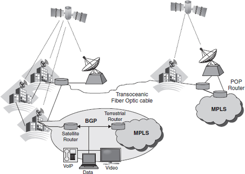
FIGURE 7.13
Satellite–cable global distribution architecture
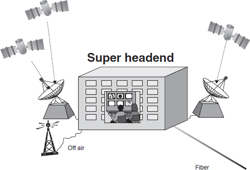
FIGURE 7.14
The Super Headend: satellite–cable distribution topology
Distribution protocols
Not all network routing protocols are suitable for TV content transmission. The selection of protocols used on a network has an impact on file transfer performance. Among the frequently used protocols are Border Gateway Protocol (BGP), MPLS, ATM, and DTM.
Border gateway protocol
The BGP (RFC 1771) is a protocol used for exchanging routing information between autonomous systems. An autonomous system is a network or group of networks that use the same routing policies and are administered as a group. Routes learned using BGP have attributes that are used to determine the best route to a destination.
In Figure 7.14, we can see that there are a number of routes that can be used to transport data from source to destination. All nodes in the network use BGP. The exchange of network metrics and routing information enables decisions to be made by network interconnection devices that will select the best path for the data transmission.
Multiprotocol label switching
MPLS is a packet-switched protocol that aids in maximizing network performance and is interoperable with IP, ATM, Ethernet, and Frame-Relay network protocols. Improved transfer speeds are attained by setting up a defined path for a sequence of packets.
The entry and exit points of an MPLS network are called label edge routers (LERs). An MPLS header containing a label is added when a packet enters the MPLS network and is removed when the packet exits. Label switch routers (LSRs) perform routing based on the label.
LSRs examine a label lookup table to determine where to switch the packets. The next hop selection operation takes place within the switched fabric and not in the router's CPU. MPLS can be considered as a combination of Layer 2, packet switching, and Layer 3, determining next hop via a lookup table for a switched path. Label Distribution Protocol (LDP) facilitates label distribution between LERs and LSRs. LSRs regularly exchange label and reachability information.
Label switch paths (LSPs) can be used to create network-based IP virtual private networks or to route traffic along specified paths through the network. LSPs are analogous to permanent virtual circuits (PVCs) in ATM or Frame-Relay networks but are independent of a particular Layer 2 technology.
Frame relay
Frame relay is a data link (Layer 2) packet-switched network protocol. It was developed as an extension of Integrated Services Digital Network (ISDN) and X.25 packet-switching technology. The driver behind its development was to find a way to transport circuit-switched protocols over packet-switched networks.
Network providers implemented frame relay for voice and data. Frame relay uses packet encapsulation over a dedicated connection. Data enters a Frame-Relay network over a connection at a Frame-Relay node.
Frame relay places data in variable-size units called “frames” and leaves error correction (such as retransmission of data) up to the end points. The structure of a basic Frame Relay frame is shown in Figure 7.15.
In 1990, Cisco Systems, StrataCom, Northern Telecom, and Digital Equipment Corporation developed a set of Frame-Relay enhancements called the local management interface (LMI). The LMI adds extensions for managing internetworks, including:
![]() global addressing;
global addressing;
![]() virtual circuit status messages; and
virtual circuit status messages; and
![]() multicasting.
multicasting.
Figure 7.16 shows the structure of an LMI Frame relay frame.
Frame-relay devices fall into two broad categories: data terminal equipment (DTE) and data circuit-terminating equipment (DCE). DTEs are typically located on the premises of a customer. Terminals, personal computers, routers, and bridges are examples of DTEs. DCEs are carrier-owned internetworking devices. Figure 7.17 shows the relationship of each type of device to the network topology.
Frame-Relay networks transfer data over connection paths referred to as virtual circuits (see Figure 7.18). There are two types: switched virtual circuits (SVCs), which are temporary; and PVCs.
The Data Link Connection Index (DLCI) is a number assigned to each virtual circuit and DTE device in the Frame-Relay network. Two different devices are assigned the same DLCI within Frame-Relay network—one on each side of the virtual connection.
ATM
ATM partitions data traffic into small fixed-sized cells intended to transport real-time video and audio. The International Telecommunications Union and the ATM Forum facilitated the creation of ATM standards.

FIGURE 7.15
Structure of a Type I Frame Relay frame
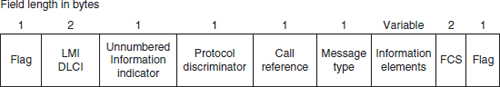
FIGURE 7.16
Structure of an LMI Type II Frame Relay frame
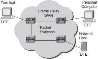
FIGURE 7.17
Typical network locations of DCE and DTC frame relay equipment
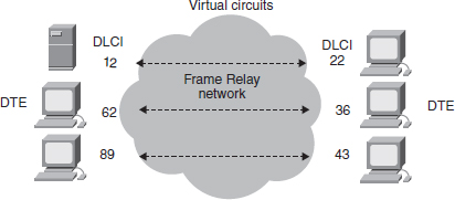
FIGURE 7.18
Frame Relay Virtual circuits
A connection-oriented technology, ATM establishes a virtual circuit between the two end points before the data transfer begins. ATM is a cell-relay, packet-switching protocol. It is a core protocol used in SONET/synchronous digital hierarchy (SDH) backbones.
ATM uses small data cells, a 48-byte payload and a 5-byte routing header, to reduce jitter (delay variance) over a network. Reduction of jitter and end-to-end delays are important for transport of real-time signals. Buffer design and size is simplified.
ATM can build virtual channels (VCs) and virtual paths (VPs). A VC uses a unique virtual channel identifier (VCI) encoded in the cell header to enable communication between two end points. A VP is a group of VCs that connect the same end points. VPs are identified by a virtual path identifier (VPI), encoded in the cell header.
ATM includes a mechanism to guarantee that “quality of service” (QoS) is maintained. QoS attributes include bit rate, packet jitter, network latency, and reliability. There are four basic types:
2. VBR: variable bit rate
3. ABR: available bit rate
4. UBR: unspecified bit rate
Modern network management systems do not allow data rates to exceed contract limits. If this should occur, the network will either drop the cells now or flag the cell loss priority (CLP) bit for discard later in the transmission path.
DTM
DTM is a high-speed network architecture based on fast circuit switching. The packet-based protocol provides guaranteed bandwidth. The packets to be transferred are separated from other network traffic and then routed over a dedicated channel that is established between transmit and receive locations.
DTM divides fiber capacity into bandwidth intervals and can provide more band-width as it is needed during the transfer operation. Other circuit-switched networks, such as SONET/SDH, are unable to adjust bandwidth during a data transfer session.
Switches, rather than routers, are located at network connection points. All processing and buffering is implemented in a silicon-based switch core using application-specific integrated circuit (ASIC) devices.
Content Backhaul Over the Internet
Internet delivery of content in broadcast operations is restricted to nonreal-time applications. Segments produced by “backpack” journalists in the field and commercial spots from agencies are often delivered to broadcast operation centers via the Internet. Another suitable workflow is graphics distribution to affiliates from a centralized production location or from a production service.
SONET and SDH
As optical data transmission technology became progressively more reliable and the need arose to increase data capacity and data transfer rates, commercial carriers (AT&T in the 1970s, MCI in the 1980s) began to install fiber-optic cables in their long-haul networks. In an effort to optimize performance, protocols specific for optical transmission were developed. SONET and SDH are multiplexing protocols for transferring multiple bitstreams over the same optical fiber.
SDH was standardized (G.707 and G.708) by the International Telecommunication Union (ITU). SONET is specified in T1.105 by the American National Standards Institute. SONET is used in the United States and Canada, while SDH is used in the rest of the world.
SONET and SDH are circuit switched. Each circuit has a CBR and delay. Both are TDM, physical layer (Layer 1) protocols utilizing a permanent connection.
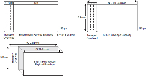
FIGURE 7.19
SONET frame structure
Table 7.2 SONET Signal Bit-Rate Capacity |
||
Level |
Bit rate (Mbps) |
Multiplex capacity |
STS-1, OC-1 |
51.840 |
28 DS1s or 1 DS3 |
STS-3, OC-3 |
155.520 |
84 DS1s or 3 DS3s |
STS-12, OC-12 |
622.080 |
336 DS1s or 12 DS3s |
STS-48, OC-48 |
2488.320 |
1344 DS1s or 48 DS3 |
STS-192, OC-192 |
9953.280 |
5376 DS1s or 192 DS3s |
STS-768, OC-768 |
39813.12 |
21504 DS1s or 768 DS3s |
The basic frame format is two dimensional and illustrated in Figure 7.19. Eighty-seven payload bytes combined with three transport overhead bytes make a 90-byte row. Nine rows make a frame.
Table 7.2 lists the bit rates used by SONET. SDH has a similar hierarchical bit-rate structure but with slightly different data rates. The difference is due to the fact that each protocol was derived from the regional telephone system.
As of 2007, OC-3072 is under development and will support 159.25248 Gbps data rates.
A SONET and SDH multiplex is built by using optical combiners. The combiners can be connected in many ways. Figure 7.20 shows a number of configurations that use signal formats discussed earlier in this chapter.
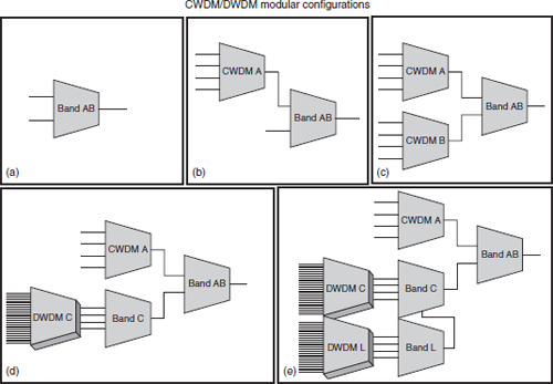
FIGURE 7.20
SONET multiplexing, CWDM/DWDM modular configurations
SONET technology can be deployed in any of the popular physical layer architectures as shown in Figure 7.21.
The ring architecture is used extensively in MANs and WANs. It offers resiliency in dual connections between add/drop multiplexers (ADMs) and has an innate backup route if the primary link fails.
SONET and SDH are multiplexes of light at various wavelengths, sometimes referred to as colors. An ADM does exactly what its name describes. A particular wavelength of light is filtered out of the multiplex; that is, it is dropped. Another signal, at the same wavelength, is added to the multiplex.
NETWORK TOPOLOGY
The network topology of the commercial carriers and the Internet can be pictured as layers, known as tiers of service. A definition of internetwork “tiers” has never been established by a standards setting body. Definition of each tier is based on financial considerations for network access.
![]() Tier 1: a network that can reach every other network on the Internet without purchasing IP transit or paying settlements. Primary carriers over SONET are AT&T, MCI, and Sprint.
Tier 1: a network that can reach every other network on the Internet without purchasing IP transit or paying settlements. Primary carriers over SONET are AT&T, MCI, and Sprint.
![]() Tier 2: a network that peers with some networks, but still purchases IP transit or pays settlements to reach at least some portion of the Internet. Examples are Level 3, Intelsat, Eurovision, and Ascent Media.
Tier 2: a network that peers with some networks, but still purchases IP transit or pays settlements to reach at least some portion of the Internet. Examples are Level 3, Intelsat, Eurovision, and Ascent Media.
![]() Tier 3: a network that solely purchases transit from other networks to reach the Internet. This tier includes typical ISPs such as EarthLink and AOL.
Tier 3: a network that solely purchases transit from other networks to reach the Internet. This tier includes typical ISPs such as EarthLink and AOL.
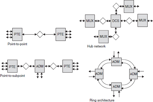
FIGURE 7.21
SONET architectures
Geographic topology and reach
Another approach to network conceptualization is based on geography. The most localized networks are LANs. As the area covered by a network expands to a metropolitan area, the network is called, naturally, a metropolitan area network (MAN). Long-haul networks that connect MANs and cover wide geographical areas are wide area networks (WANs).
Figure 7.22 illustrates the general hierarchical topology of network categories.
Although a formal definition does not exist, LANs are generally confined to an office, building, or part of an organization. The network architecture, routing protocols, and network bandwidth are also defining characteristics. LANs were usually 10/100 Mbps, but GigE is becoming more frequently deployed to the desktop. In the media production world, GigE is ubiquitous. A LAN can be considered an autonomous system.
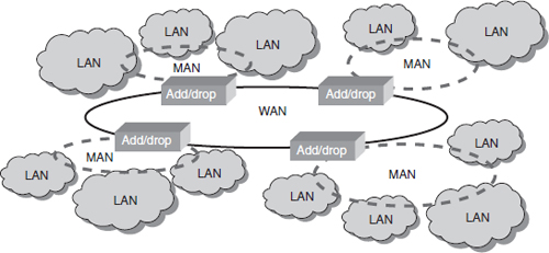
FIGURE 7.22
Network topologies (internal LAN and external WAN)
MANs and WANs are optical networks. Data rates of 10 Gbps and higher are common on MANs, while WANs are now reaching 40 Gbps with 100 Gbps in the development and test stage.
In the United States, SONET-based optical networks form the backbone of many public and private networks. As can be seen in Figure 7.23, installed fibers are densest in large metropolitan areas and the MANs are hard to see. The larger lines that cross the country are the WAN backbone.
Telco TV
Telcos now are leveraging their distribution plants to deliver DTV, either over a dedicated IP broadband line or over fiber optics. Each technology used is proprietary. AT&T uses fiber-to-the-node (FTTN) for IPTV, while Verizon uses fiber-to-the-home (FTTH) and calls their technology FiOS.
Figure 7.24 shows a typical IPTV system architecture. Content for national distribution is aggregated at a national headend. The IP core network is a WAN and traverses large distances on a national scale. The IP core moves content to regional headends over a metro aggregation network, a MAN. Access nodes connect to the MAN. Content is transferred over the last mile from the access node, sometimes called a central office, to the customer. As can be seen, this distribution network architecture closely follows the WAN/MAN/LAN model.
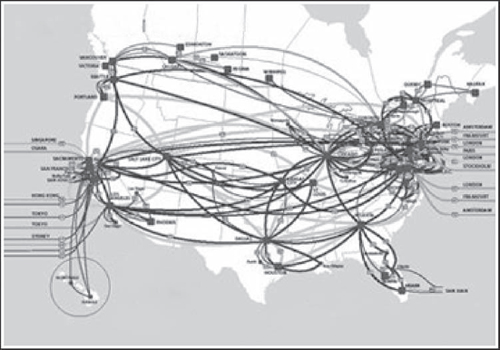
FIGURE 7.23
Typical national WAN backbone
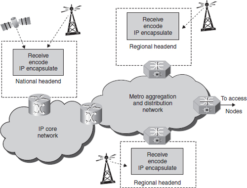
FIGURE 7.24
IPTV system architecture
Cellular backhaul
Mobile communications has been around almost as long as radio itself. Starting from 1950s, two-way radios were used in civil service vehicles such as taxicabs, police cruisers, and ambulances. The 1970s saw the consumer adoption of citizens’ band radios most often used by truckers. These were all closed systems, not connected to the telephone network, but specifically suited to their purpose: reliable communication.
In time, the need to make calls from a vehicle led to mobile phones that were permanently installed in vehicles.
During the early 1940s, Motorola developed a backpacked two-way radio, the walkie talkie, and later developed a large handheld two-way radio for the U.S. military.
Mobile phones became a mainstream device over the last decade. Delivery of video either as a broadcast or as cell-based content is an evolving technological capability.
As systems grew in geographic scope, backhaul methods were needed to route calls across the country. This necessitated connecting to the public-switched telephone network: landlines.
Existing cell phone backhaul networks were originally designed for voice communications. Network topology was based on data rates of 3 kHz voice data. As features that required data capabilities emerged, improvements to the backhaul networks were made where necessary.
Consumer desire to connect with the Internet and receive video on cell phones changed everything. Even highly compressed video and audio are an order of magnitude more demanding than voice channel data capacity. This led to the development and deployment of 3G distribution to consumers and large-scale upgrades of the cellular backhaul infrastructure.
Optical backhaul over SONET networks provided a limited solution. Figure 7.25 illustrates a typical long-haul network.
Data rates of digital telephone lines were too small for the available video compression capabilities at the time and prohibited real-time delivery of TV programming. As cell phone subscribers increased, and call volume exceeded available network capacity, quality was reduced by leveraging statistical multiplexing. In addition, multiple services were aggregated over a unified transport. This topology could never support real-time video applications.
As IP-based packet transport capacities have improved, the original connection-based SONET transport networks have been supplemented by a packet transport network.
In some scenarios, the Internet can be used for nonreal-time video distribution. A typical topology is shown in Figures 7.26 and 7.27.
The three-tiered network topology is leveraged once again. Content aggregated at the national level is distributed to local operation centers. There it is supplemented with locally originating content. From there it is distributed to the tower infrastructure.
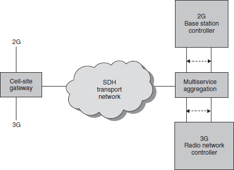
FIGURE 7.25
2G and 3G cellular backhaul optimization
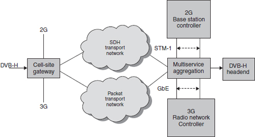
FIGURE 7.26
Cellular DVB-H backhaul integration example: SDH to packet migration scenario
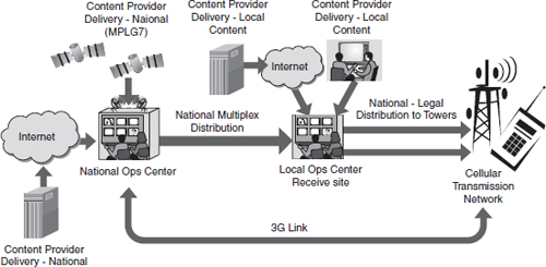
FIGURE 7.27
Cell phone content aggregation and backhaul for store and forward content distribution
THE BEST IT CAN BE
In this chapter, the movement of content between broadcast segments was described for each of the distribution networks that support a three-screen universe. The point is to emphasize the differences between professional content delivery networks and consumer distribution. As DTV screens get larger and larger, and programming uses content from many nontraditional sources, viewers will no longer tolerate low-quality presentations.
The “garbage in, garbage out” adage fits to some extent—How do you improve the quality of less-than-broadcast-quality content? At the other end of the spectrum, content produced for television employs high production values. Content distribution networks strive to deliver this content in as high a quality as possible.