
|
|
Chapter 7
|

Dimension modeling is a logical design technique that seeks to present the data in a standard framework that is intuitive and allows for high-performance access.
Ralph Kimball (Kimball 2008)
When you have completed this chapter, you will be able to:
• Understand dimensional modeling terms
• Apply data modeling to business intelligence
• Design a data mart using dimensional modeling.
In Chapter 7, you learned to model the data as it is extracted, cleansed, and integrated in preparation for loading to the data mart. In this chapter, you will understand how to arrange data for delivery to the user – the people who analyze the data.
The following dimensional modeling topics will be explained:
• Top Down / Requirements Driven Approach
• Fact Tables and Dimension Tables
• Multidimensional Model / Star Schema
• Roll Up, Drill Down, and Pivot Analysis
• Time Phased / Temporal Data
• Operational Logical and Physical Data Models
• Normalization and Denormalization
• Model Granularity – the Level of Detail.
Areas that require specialized patterns are:
• Staging / Landing Area – looks like source system
• Data Warehouse – uses normalized ERD
• Data Mart – uses dimensional modeling – the ROLAP star schema or the MOLAP cube.
Dimensional Data Modeling
The best way to organize data is to meet the needs of its users. Business intelligence commonly performs analytic operations on data. These operations are described in more detail in Chapter 12, Business Intelligence Operations. They include the following:
• Query by multiple criteria – The analyst explores data and focuses the search on specific areas of interest. For example, the analyst may use sales territory and product as criteria for data selections.
• Drill down – The analyst explores data at a more detailed level. For example, the analyst may start analysis of sales figures summarized by sales territory, then drill down to the store level, and even further to individual sales transactions.
• Roll up – The analyst explores data at a summarized level. This is the reverse of Drill Down. For example, sales could be rolled up from the territory level to the region level.
• Slice and dice – The analyst explores data by focusing on a specific dimension, such as sales territories or products.
The “Dimensional Data Model” was popularized by Ralph Kimball and others in the 1980s to support business needs for analytical operations. This approach has stood the test of time and is the recommended way to organize data for business query and analysis.
The dimensional model provides a number of benefits including:
• Maps to business process – The measures correspond to business activities such as sales, manufacturing, and accounting.
• Ease of query – Data is organized so that analysts can easily query information, which enables operations like drill down and roll up.
• Ease of modification – The data is organized so that changes can be made to the database design, such as the addition of new attributes.
• Efficiency of query – Data is organized so that it can be accessed quickly by computer. For example, data is stored using surrogate keys, which enable highly efficient data access.
• Support by query tools – BI tools are designed to access data that is stored in dimensional format.
• Understandable design – The arrangement of data in the dimensional format is easy to understand because it builds on the well understood paradigm of cubes and analytical operations.
The basic terms describing the dimensional model are described in Table 07-01.
Table 07-01: Data Mart Basic Model
|
Term |
Definition and Description |
|
Data Mart |
A data mart is a database in which data is stored to ensure good performance for presentation and user access. Early definitions specified that data marts were targeted to specific subjects and business processes. In practice, the data mart is a database that is organized into facts and dimensions that can cross subjects. |
|
Fact |
A fact is a set of measures. It contains quantitative data that are displayed in the body of reports. It often contains amounts of money and quantities of things. In the dimensional model, the fact is surrounded by dimensions which categorize the fact. |
|
Dimension |
A dimension is a database table that contains reference information to identify and categorize facts. The attributes serve as labels for reports and as data points for summarization. In the dimensional model, dimensions surround and qualify facts. |
|
Hierarchy |
A hierarchy is an arrangement of entities into levels where each entity has one parent and may have multiple children. A geographic hierarchy could have levels such as: continent, country, state, county, city and postal code. |
|
Cube |
A cube is a data structure organized into dimensions, measures, and cells. Cubes contain a set of detailed measures at the leaf-level, for each distinct combination of dimensions, plus aggregated measures for roll ups where one or more dimensions are removed from a hierarchy. |
|
Metric |
A metric is a direct, quantified measure of performance, such as revenue, cost, unit sales, and complaint count. |
|
Cell |
A cell is a set of measures associated with a distinct set of dimensions within a cube. Empty cells contain no data for a particular combination. |
Star Schema
A Star Schema is a database that is optimized for query and analysis. It is a form of dimensional model consisting of facts and dimensions, where each fact is connected to multiple denormalized dimensions that are not further categorized by outlier dimensions. It is a straight forward dimensional model.
The two major table types of the Star Schema are the fact table and the dimension table. The fact table contains quantitative measures, while the dimension contains classification information. Each fact is surrounded by the dimensions that provide context to it, giving it the appearance of a star, as depicted in Figure 07-01.
Figure 07-01: Star Schema – A Fact Surrounded by Dimensions

The Sales Order Fact with dimensions, shown in Figure 07-02, is a classic example. In this case, the Sales Order Fact includes the measures order quantity, and currency amount. Dimensions of Time Period, Product, Customer, Geo Location, and Sales Organization put the Sales Order Fact into context. This star schema supports looking at orders like a cube, enabling slicing and dicing by customer, time, and product.
Figure 07-02: Sales Order Star Schema

The Star Schema, fact tables with their associated dimensions, is oriented to describing and measuring business processes and answering critical questions. Figure 07-03 shows that dimensions typically answer descriptive questions such as: where, when, why, how, who, and what. Facts answer quantitative questions such as how much and how many.
Figure 07-03: Star Schema is Oriented to Answering Questions

The order process is an example of what may be measured using a star schema. Use of business process analysis methods such as SIPOC (Suppliers, Inputs, Processes, Outputs, and Customers) is a great way to get a handle on the requirements for a star, as depicted in Figure 07-04.
Figure 07-04: Analytical Data Supports Business Processes

Example Star Schema
Understanding the star schema requires a deeper dive. In the Figure 07-05 example, each table follows a naming convention with a prefix of “DM_” for Data Mart, a suffix of “_Dim” for dimension names, and facts have a suffix of “_Fact”.
Each dimension has a primary key that uniquely identifies the dimension. This primary key, known as a surrogate key, is system generated and used in place of the business key of the dimension.
Surrogate keys, typically stored as integers, improve efficiency and increase performance. Database joins between facts and dimensions are faster with integers. Indexes on integers are compact and provide rapid access. Figure 07-05 shows surrogate keys for each of the dimensions – product, customer, sale item, and date. The DM_Product_Dim table has a primary key of dm_product_dim_id and a business key of product_code.
The primary key of the fact consists of one or more foreign keys that relate to dimensions. In this case, the primary key of the DM_Sale_Item_Fact brings together the product, customer, sale item, and date dimensions. This fact contains a single measure, the item sale_amt.
Figure 07-05: Star Schema DM_Sale_Item_Fact Example

It is now time to go to the next level and explain both facts and dimensions in greater depth.
Facts – the Data Mart Measuring Stick
Facts contain quantitative measures about the subject of analysis, typically a business process. Facts focus on answering the questions of how much and how many. Figure 07-06 provides an additional example of a fact, in this case a Sales Order Fact. The name of the fact table should describe the business process and granularity of the fact.
The primary key of the fact table is made up of foreign keys from its surrounding dimensions. These dimensions specify the grain of a single fact. Keep in mind that not all foreign keys from dimensions have to be part of the fact primary key.
Of course, data is a critical part of facts. Keep in mind what you learned about data in Chapter 5, Data Attributes, when selecting measure data to be included with the fact.
Figure 07-06: Anatomy of a Fact

Granularity
The grain is the lowest level of detail of what is measured by a single occurrence of the fact. A fact with fine granularity might contain data about a single transaction or part of a transaction, while a coarse-grained fact might contain information that summarizes multiple transactions over a period of time. Selecting the appropriate grain for each fact is a critical design decision, and should be part of the design specification for each fact.
In the data mart, atomic data is detailed data at the lowest level of granularity – it cannot be broken down further. Transactional data, such as sales, shipment, and financial transactions, are common examples of atomic data. The advantages of data at a detailed grain are that it can answer very detailed questions and it can also be rolled up into summary information. Summary information has an aggregated grain, which provides faster summarized results and requires less storage than detailed grain information.
On the downside, a very detailed grain requires more storage and more time to summarize when querying. The down side of an aggregated grain is that details may not be available for further analysis (drill down). Creating aggregated grain (summary) tables may be a little risky unless it is very clear what aggregation is needed. Otherwise, time and space could be wasted creating unused summaries when the data is populated.
Fact Width and Storage Utilization
In most data marts, facts use most of the disk space because they naturally have far more rows than dimensions. Data models make it look like dimensions are equal in size to facts. This may be true in terms of the number of attributes per table, but it is not true in terms of the total disk space used. See Figure 07-07 to get this in perspective. To conserve disk space and improve performance, fact tables should be narrow, minimizing the number of attributes needed to provide the measures the business requires. Every attribute added to a fact table is costly because it is multiplied by the large number of rows that are stored in the table.
Figure 07-07: Disk Storage Model

Mathematical Nature of Facts – Can it “Add up”?
The ability to summarize data is limited by the additive nature of the data, coupled with its grain. First, the properties of the data are examined without considering dimensions. This topic was first tackled in Chapter 5, which describes the types of data attributes – nominal, ordinal, interval, and ratio. The definitions and descriptions are repeated here in Table 07-02.
Table 07-02: Data Attribute Quantitative Categories
|
Term |
Definition and Description |
|---|---|
|
Nominal |
Nominal data names and describes. It can be evaluated for equality or inequality, but it cannot be ordered, added, or multiplied. Nominal data is usually part of dimensions, not facts. |
|
Ordinal |
Ordinal data has sequence. Data can be ranked and evaluated as being equal to, less than, or greater than other ordinal data of the same type. Ordinal data cannot be added or multiplied. The following is a typical ordinal scale:
1 = Strongly Disagree
|
|
Interval |
Interval data is numeric without a “true zero”, so the operations of division and multiplication are not applicable. Examples of interval attributes include time of day, credit scores, and temperatures measured in Celsius or Fahrenheit. |
|
Ratio |
Division and multiplication do apply to ratio data because ratio data does have a “true zero” in its scale. Examples of ratio attributes include time durations, counts, amounts, weights, and temperatures measured in Kelvin. |
The terms describing the additive nature of attributes are described in Table 07-03.
A data mart can be composed of several types of facts. Each of these types is explained in the following pages:
• Event or Transaction fact
• Snapshot Fact
• Cumulative Snapshot Fact
• “Factless” Fact.
Table 07-03: Addition Related Terms
|
Term |
Definition and Description |
|
Fully-Additive |
Fully-additive attributes can be summed across all dimensions of a fact table. These attributes are discrete numerical measures of performance. Fully-additive attributes often occur in facts that measure events. They contain information such as quantity shipped and dollars deposited. |
|
Semi-Additive |
Semi-additive attributes can only be summed across some of the dimensions of a fact table. These attributes tend to be point in time computed values such as inventory balance, account balance, and period to date activity. |
|
Non-Additive |
Non-additive attributes cannot be correctly summed for any of the dimensions of a fact. Examples of non-additive attributes include rankings, percentages, and unit price. |
Event or Transaction Fact
The most commonly utilized fact type is the event or transaction fact. This type of fact captures events, with each event record in a single row of the fact table. The grain of the table is a single event such as a financial transaction, sale, complaint, shipment, or sales inquiry. Measures for event facts are generally additive across all dimensions, subject to the guidance just provided about the mathematical nature of measurements. Figure 07-08 shows an event fact. In this model ‘txn’ is an abbreviation for transaction and ‘GL’ is an abbreviation for general ledger.
Figure 07-08: Event Fact Example

Event transactions are often at or near the atomic level. For example, a single sale may be broken into multiple sales transactions – one per line item. The dimensions associated with an event can be identified using the Kipling question model (Table 07-04 – who, what, when, where, why) and the measures by the Kipling Questions (how much, how many).
Table 07-04: Kipling Dimensional Questions
|
Term |
Definition and Description |
|
When |
When did this event occur? What was the date and time of the event? |
|
Who |
Who played the roles of worker, customer, supplier, authorizer, etc.? |
|
Why |
Why did this event occur? This could include a reason code, as well as links to plans such as campaigns, projects, and budgets. |
|
Where |
Where did the event take place? This can be a geographical breakdown, as well as an organization breakdown. |
|
What |
What products or assets are associated with the event? |
|
How |
How did this event happen? What processes or procedures are associated with the event? |
Snapshot Fact
A snapshot fact captures the status of something at a point in time. The snapshot fact captures quantities and balances effective on a specified date and is sometimes known as an inventory level fact or balance fact. The time dimension is used to identify the grain, such as monthly, quarterly, and yearly. Snapshot data is not additive across time; however, data is typically additive across the other dimensions. Examples of snapshot fact types include:
• Financial account balances
• Inventory levels
• Activity counts such as open issues.
Figure 07-09 shows a snapshot fact that contains general ledger balances. The balances are effective on a specified calendar date, for a specific account, and organizational unit.
Figure 07-09: Snapshot Fact Example

Cumulative Snapshot Fact
A cumulative snapshot fact is a variation of the snapshot fact with the addition of year to date (YTD) totals. Figure 07-10 shows an example of a cumulative snapshot fact.
Figure 07-10: Cumulative Snapshot Fact Example

Aggregated Fact
An aggregated fact is a summary of information, such as atomic facts. The aggregations are arrived at by removing one or more dimensions from an atomic level fact. The additive properties of the measures must be recognized when building the aggregated fact data. Aggregation may include count, sum, minimum, maximum, mean, and median quantities. Aggregation analytical categorization such as:
• Sales by sales rep by month
• Shipments by product by facility by week
• Complaints by product by store by month
• Downloads by category by website by quarter.
Figure 07-11 shows an aggregated fact. In this case, revenues have been aggregated by month. In this model ‘txn’ is an abbreviation for transaction and ‘GL’ is an abbreviation for general ledger.
Figure 07-11: Aggregated Fact Example

“Factless Fact”
A factless fact tracks the existence of a set of circumstances as described by dimensions, rather than a measurement of amounts or quantities. This type of fact is helpful when describing situations such as events or coverage. Examples of factless facts include milestone occurrence, event attendance, and sales promotion. Figure 07-12 shows a factless fact.
Figure 07-12: Factless Fact Example

Dimensions Put Data Mart Facts in Context
Dimensions enable business intelligence users to analyze data using simple queries. Dimensions focus on the questions of who, what, when, and where. They contain attributes that describe business entities. Typical dimensions include:
• Time Period / Calendar
• Product
• Customer
• Household
• Market Segment
• Geographic Area
• Financial Account Structures.
Dimensions are used in the query process to select, group, and order data. The attributes of an entity can be independent or can be organized into hierarchies, often with three to five levels. For example, sales organization attributes could include region, district, territory, branch, and sales representative.
Getting the number of dimensions and attributes right is an important part of dimensional design. Most facts should be associated with two to fifteen dimensions. Too few dimensions tend to be not descriptive enough, while too many dimensions are a sign that the dimensions are not structured correctly and should be combined. Placing a large number of dimension keys on a fact table increases storage space and load time.
Effective dimensions are descriptive and contain rich information. Figure 07-13 provides an example of these rich dimensions. There are often numerous attributes, fifty to one hundred or more. Data is denormalized to reduce database joins, while providing rich descriptions. Much of the data in a dimension is descriptive and stored in character format. It often contains both code and expanded values, such as mfg_location_code and mfg_location_desc, to simplify and speed up queries.
When designing dimensions, it is important to understand dimension hierarchies and the navigation paths that data mart users are likely to use. Clues to this can be found by analyzing existing reports for data groupings and summarization levels. Dimensions are supported by source data, so apply data profiling to source data to make sure that it is correct and complete in the area of hierarchies.
Figure 07-13: Rich Dimensions

Dimension Keys
There are two types of keys associated with dimensions, the surrogate key and the business key. The surrogate key is used as the primary key of the dimension, while the business key is used as an alternate key. Figure 07-14 shows a typical dimension with surrogate and business keys.
The surrogate key is typically a sequential integer without any business meaning. This key is used to join from the dimension to the fact. A single integer has been found to be very efficient and effective for database joins. In addition, fact table sizing decreases with the use of more compact integers, rather than longer text columns.
The surrogate key should be generated within the data mart. Keys from source systems should be avoided because they could change in the source system, resulting in a mismatch with the data mart. Use of smart keys, which have embedded meaning, should also be avoided.
The business key does include human identifiable information such as purchase order number, credit card number, and account code. It consists of one or more columns that identify a distinct instance of a business entity. An effective date may be part of a business key, as described in SCD Type 2. Figure 07-14 illustrates the use of a surrogate key (product_key) and a multiple column business key (product_nbr, product_ver_nbr, dm_effective_date).
Figure 07-14: Dimension Keys

Data Modeling Slowly Changing Dimensions
At times, the data mart must handle changes to dimension. Ralph Kimball has identified the following slowly changing dimension (SCD) types that are widely recognized in data mart design:
• SCD Type 0: Data is non-changing – It is inserted once and never changed.
• SCD Type 1: Data is overwritten and prior data is not retained.
• SCD Type 2: A new row with the changed data is inserted, leaving the prior data in place.
• SCD Type 3: Update attributes within the dimension row. For example, both current customer status code and prior customer status code could be maintained.
SCD Type 0 – Unchanging Dimensions
Slowly changing dimension type 0 is used when changes made to the source system should not result in any updates to the dimension and no maintenance of history is required. This can be used for static tables such as dates. In this case, rows are inserted once, but never updated.
SCD Type 1 – Overwrite
Slowly changing dimension type 1 is used when changes made to the source system result in an update to the dimension without maintaining a history of earlier values. This makes sense when source system changes are corrections or have no significance. Figure 07-15 shows the RatingCode in the data source has changed from “BBB” to “AAA”. In the data mart, the RatingCode also changes from “BBB” to “AAA”. The data mart shows only the current value and does not show the change.
Figure 07-15: SCD Type 1 Example

SCD Type 2 – New Row
Slowly changing dimension type 2 is used when changes made to the source system should result in saved history in the data mart. This is used when changes to the source system are true changes in meaning and significance. Typically, an effective date is part of the dimension table and the business key. A new row is inserted, with a new effective date, matching business key, and changed data. This approach preserves the earlier data. Figure 07-16 shows the RatingCode in the data source has changed from “BBB” to “AAA'. In the data mart, the existing row is expired by changing DWEndDate to “2004-04-09” and then inserting a new row with the changed value.
Figure 07-16: SCD Type 2 Example

Figure 07-17: SCD Type 3 Example

SCD Type 3 – New Column
Slowly changing dimension type 3 is used when there is a transition of values in the source system. An example of this would be adding a new department name. SCD Type 3 maintains current and old versions of the changing columns. An effective date that is specific to the updated column may also be included. Figure 07-17 shows an additional column, RatingCodeOld, which contains the prior value of RatingCode.
In this case the source system changes RatingCode from “BBB” to “AAA”. In the data mart there is an update where RatingCodeOld is set to “BBB”, the prior value of RatingCode, and RatingCode is set to “AAA”. Note that only the most recent change is available. If the rating code changed again at a later date, Rating Code Old would become “AAA” and Rating Code would contain the new value.
Date and Time Dimension
Date and time dimensions are an important part of almost every dimensional model. I recommend that you establish date and time of day dimension tables rather than use hard coded date logic. A date dimension is often organized into days and accounts for days of the week, weeks, quarters, seasons, holidays, etc. Figure 07-18 shows example date and time dimensions. The date_key can be a smart integer key such as 20120103 (yyyymmdd) or non-smart key such as 140789 to represent January 3rd, 2012. Use of the smart date key avoids the need to join to the date_dim table for simple dates, however, an unknown date represented as 99999999 must be treated an exception. Smart keys could also be used for the time of day dimension such as 180403 (hhmmss) to represent 6:04:03PM.
Figure 07-18: Date Dimension and Time of Day Dimensions

The Time of Day Dimension captures the time during the day and is useful for gaining an understanding of business volume questions. For example, time of day could be captured for ATM transactions in a fact which references the time of day dimension to learn when peaks and valleys occur.
One Dimension – Multiple Roles
At times, one dimension may be related in multiple ways to the same fact. This often happens with the Calendar Date Dimension and the Party Dimension. Figure 07-19 shows an example of how a dimension may have multiple relationships to a fact. Project Snapshot Fact, could be related to a Calendar Date Dimension for snapshot date, start date and end date. A project could be related to Party Dimension for project manager and project sponsor.
Figure 07-19: Multiple roles for a Dimension

Snowflake Schema
The snowflake schema as shown in Figure 07-20 is an extension to a star schema, intended to reduce storage and duplication. Instead of all dimensions being directly associated with facts, it allows dimensions to be associated with other dimensions. This is a normalized approach that reduces duplication. It can make hierarchies explicit and is very flexible.
Unfortunately, the snowflake also has undesirable consequences. It can make it queries more difficult and complex, and slow performance because more joins are required.
Use of the snowflake to reduce storage cost is an advantage. Since dimensions often account for less than five percent of space, this advantage usually is of minor importance.
Figure 07-20: Snowflake Schema

Dimensional Hierarchies
Dimensions are often used to express hierarchies, which are arrangements of entities that are organized into levels where each entity has one parent and may have multiple children. Some hierarchies have a fixed number of levels, while others have an open ended number of levels. Figure 07-21 shows two hierarchy examples, a calendar hierarchy and a sales hierarchy.
Figure 07-21: Dimensions Support Hierarchies

Figure 07-21 shows hierarchies that can be expressed through a single dimension with specific attributes. The sales hierarchy is broken into levels: region, district, sales representative, and consumer. A hierarchy where each level is filled in is known as a balanced or smooth hierarchy. The world is not always so simple. The layout of hierarchies can change over time.
A general purpose alternative is the hierarchy helper approach, as shown in Figure 07-22. The columns that make up a hierarchy helper are described in Table 07-05. This approach allows for a virtually unlimited number of levels, including ragged hierarchies, which are hierarchies that can have variable depth and missing intermediate levels. The drawback is that queries and loading are more complicated for this type of hierarchy.
Figure 07-22: Hierarchy Helper

Table 07-05: Product Hierarchy Helper Attributes
|
Attribute Name |
Attribute Description |
|---|---|
|
product_hierarchy_helper_key |
The primary key of the product_hierarchy_helper table. |
|
parent_product_key |
Foreign key to the next higher level product dimension. |
|
child_product_key |
Foreign key to the next lower product dimension. |
|
parent_top_ind |
An indicator that specifies whether the parent is at the highest point of the hierarchy. |
|
child_bottom_ind |
An indicator that specifies whether the child is at the lowest point in the hierarchy. |
|
dm_effective_date |
Date when this helper relationship started to be effective. |
|
dm_expire_date |
Date when this helper relationship stopped being effective. |
|
parent_level_nbr |
The position of the parent product in the hierarchy with level 1 being the top of the hierarchy. |
|
parent_child_distance_nbr |
A count of the levels between parent and child products. |
|
hierarchy_report_seq_nbr |
The sequence in which this relationship should be included in hierarchy reports and displays. |
Three patterns for expressing hierarchies are shown in Figure 07-23: star schema snowflake schema and hierarchy helper.
Figure 07-23: Hierarchy Example Comparisons

Bridge Tables Support Many to Many Relationships
A bridge table supports a many to many relationship between facts and dimensions. For example, a bridge table could show the percentage commission split between multiple sales reps (dimension) and a sale (fact) as shown in Figure 07-24.
Figure 07-24: Bridge Table Linking Fact and Dimension

Degenerate Dimension
A degenerate dimension consists of a dimension key without a supporting dimension table. Operational control numbers such as transaction number, shipment number, and order number are added to a fact. This number provides valuable information and can be traced back to a source system. Figure 07-25 shows an example of the use of a degenerate dimension.
Figure 07-25: Fact with Degenerate Dimension

Profile Dimension
The profile dimension contains a cluster of related characteristics such as customer behavior or customer engagement. Figure 07-26 shows an example of profile dimensions. The behavior profile describes what an individual does, while the demographics profile describes who an individual is. Use of profiles enables discovery of patterns. In addition, it saves storage space because the profile data is stored less often than it would be if stored for each customer. The demographics and behavior profile dimensions could be directly related to the customer dimension or they could be related to customers via facts.
Figure 07-26: Profile Dimension

The clusters discovered through statistics and data mining are candidates to be rows in profile dimensions. Clusters are groupings of data points with a large degree of affinity. The data points within a cluster are closer to other members of the cluster and farther away from members of other clusters.
Clusters can be given names and may be used for customer analysis. Analytic data suppliers such as Acxiom supply customer life style information organized into clusters.
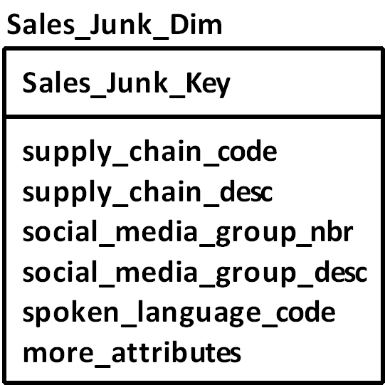
Junk Dimension
The junk dimension is a table that groups multiple unrelated attributes with the goal of reducing the number of dimensions which results in saving storage space and multiple joins. In addition, the junk dimension avoids placing miscellaneous descriptive information on facts. Figure 07-27 shows an example of a junk dimension.
Figure 07-27: Junk Dimension
Specifying a Fact
What should be included when specifying a fact? I recommend developing and using a standard template that covers the basic factors of fact design. Figure 07-06 illustrates the specification of the Sales Shipment Transaction Fact.
Table 07-06: Fact Specification Template
|
Fact Name |
Sales Shipment Transaction Fact |
|
Business Process |
Customer Order Fulfillment |
|
Questions |
How much of product X did we ship in May 2012? |
|
Grain |
Individual customer shipment transaction |
|
Dimensions |
Date, Customer, Product |
|
Measures |
Shipment quantity |
|
Load Frequency |
Daily |
|
Initial Rows |
55,000 |
The elements of the fact specification include:
• Fact Name – A fact name is a string that identifies and describes a fact in the data mart
• Business Process – The names of the business activities or tasks associated with the fact
• Questions – A list of questions that the fact will be used to answer
• Grain – A description of the level of detail or summarization represented by a single fact
• Dimensions – A list of the dimensions associated with the fact
• Measures – The quantitative characteristics associated with the fact such as counts and amounts
• Load Frequency – A specification of the timing of the population of the fact, such as daily, weekly, or hourly
• Initial Rows – The number of entries that will be populated in the fact table when it is first created.
Specifying Data Mart Attributes
Use of a template to define each attribute is also useful. Table 07-07 illustrates elements that are helpful in specifying the data attributes.
Table 07-07: Attribute Specification Template
|
Attribute Name |
YTD Deposit Amount |
|
Datatype |
decimal(11,2) |
|
Domain |
money |
|
Initial Value |
zero |
|
Rules |
This amount is reset to zero at the start of each year. |
|
Definition |
The monetary amount that has been deposited in an account from the beginning of the current year until the present. |
The attributes are described as follows:
• Attribute Name – An attribute name is a string that identifies and describes an attribute. Each attribute has a name, such as Account Balance Amount.
• Datatype – This is the format used to store the attribute. It specifies if the information is a string, a number, or a date. In addition, it specifies the size of the attribute. The datatype is also known as the data format. An example of a value is decimal(12,4).
• Domain – A domain is a categorization of attributes by function; for example Money.
• Initial Value – An initial value such as 0.0000 is the default value that an attribute is assigned when it is first created.
• Rules – Rules are constraints that limit the values that an attribute can contain. For example, “The attribute must be greater than or equal to 0.0000.” The use of rules helps to improve the quality of our data.
• Definition – An attribute definition is a narrative that conveys or describes the meaning of an attribute. For example, “Account balance amount is a measure of the monetary value of a financial account such as a bank account or an investment account.”
The meaning and usage of specialized data mart attributes are described in Table 07-08. “Audit attributes” track the dates when information was inserted or expired.
Table 07-08: Specialized Data Mart Attributes
|
Attribute Name |
Attribute Description |
|
assigned_key |
A Data Mart assigned surrogate key. The convention followed in this book is the name of the assigned key includes the name of the table with the suffix removed. For example, the assigned key of Product_Dim is Product_Key and the assigned key of Campaign_Dim is Campaign_Key. |
|
dm_insert_date |
The date and time when a row was inserted into the data mart. |
|
dm_effective_date |
The date and time when a row in the data mart became active. |
|
dm_expire_date |
The date and time when a row in the data mart stopped being active. |
|
dm_data_process_log_id |
A reference to the data process log, which is a record of the process that loaded or modified data in the data mart. |
The Big Picture – Integrating the Data Mart
To build an understanding of the enterprise requires linking our facts together to perform root cause analysis and enable drill across. This is accomplished by defining and sharing common dimensions between facts. These dimensions, known as conformed dimensions, are designed to mean the same thing when attached to multiple facts. Figure 07-28 shows example star schemas before they have been related using conformed dimensions.
Figure 07-28: Stars and Integration

A conformed dimension is a consistently defined dimension that qualifies multiple facts. For example, a product dimension could qualify both a sale_fact and a customer_feedback_fact. A conformed dimension is used to link multiple facts, build federated data marts, and support drill across. Examples of candidate conformed dimensions include:
• Product Dimension
• Customer Dimension
• Geographic Dimension
• Date Dimension.
Data Warehouse Bus
Use of the Data Warehouse Bus, an innovation by Ralph Kimball, takes the conformed dimension to the next step. A data warehouse bus is a method of coordinating data marts by matching conformed dimensions to facts. This method promotes drill across. Figure 07-29 shows an example of a set of conformed dimensions, arranged in a bus-style that connects multiple facts.
Figure 07-29: Data Warehouse Bus Summary Data Model

Another way to describe and document the data warehouse bus is through use of a table that relates the facts and dimensions as depicted in Table 07-09. This is the clearest and most compact way to describe and document the data warehouse bus. For example, the Inspection Fact is connected to the Date, Product, and Geography dimensions. In addition, the Date, Product and Geography dimensions are connected to all of the facts. It would make sense to implement these shared dimensions before implementing the Sales Rep and Customer dimensions, which are not shared.
Table 07-09: Data Warehouse Bus Table
|
Fact/
|
Sales Rep Dimension |
Customer Dimension |
Date Dimension |
Product Dimension |
Geography Dimension |
|
Inspection Fact |
|
|
x |
x |
x |
|
Production Fact |
|
|
x |
x |
x |
|
Receipt Fact |
|
|
x |
x |
x |
|
Order Fact |
x |
x |
x |
x |
x |
|
Shipment Fact |
x |
x |
x |
x |
x |
The data warehouse bus is an excellent design, planning, and communication tool. As a design tool, it helps in laying out the data mart – deciding on the specific dimensions needed to make the system produce good analytic results. As a planning tool, it enables determination of dependencies. It shows which dimensions must be in place to support which facts. In addition, it becomes easier and faster to implement facts as more dimensions are implemented. It is a matter of attaching existing dimensions, rather than creating new dimensions. Finally, it is a great communication tool. This straightforward chart is an understandable way to talk through the structure of the data mart with stakeholders.
The Bigger Picture – The Federated Data Mart
Organizations often have multiple data warehouses and data marts, which leads to an integration challenge. These data marts may have been acquired as turnkey systems, created for department and division applications, or through an acquired business. Benefits could be realized by integrating this data, but developing an overall data warehouse may be expensive and time consuming.
One answer is the federated data warehouse, which is a data warehouse system that uses virtual methods to consolidate multiple underlying data warehouse and data mart databases. It is used to produce a unified view of data and improve speed to market. The virtual method approach does not physically combine the data. Instead, data is related through a virtual schema which makes it appear as a single data warehouse to its users. This approach was introduced in Chapter 4, Technical Architecture. The database technology is further described in Chapter 11, Database Technology.
Data in the virtual schema is integrated through conformed virtual dimensions. This is based on matching logical keys between systems. For example, customer number can be used to integrate customer data.
|
Key Points • The star schema, the key structure of the dimensional model, is where a fact table is connected to multiple dimension tables. • A fact is a set of numeric measures, such as money and quantities of things. • Dimension tables provide context in the form of descriptive data that is used as labels on reports or filters for analysis. • A dimension that consistently qualifies a number of facts is called a conformed dimension. This supports analysis that requires linking of facts, plus reduces costs by reducing duplication. • Slowly changing dimensions (SCDs) are dimensions where the logic key is constant and non-logical key data may change overtime. These SCDs are categorized into types one through three, with each type having its own approach to recording change. |
Learn More
Build your know-how in the area of dimensional modeling using these resources.
|
Read about it! |
There are numerous books that describe dimensional modeling. These are some of the best: Kimball, Ralph and Associates. The Data Warehouse Lifecycle Toolkit. Wiley, 2008. Adamson, Christopher. Star Schema The Complete Reference. McGraw-Hill Osborne Media, 2010. |