4

Understanding Customer Preferences with Conjoint Analysis

Conjoint analysis is a well-known approach to product and pricing research that identifies customer preferences and makes use of that knowledge to choose product features, evaluate price sensitivity, anticipate market shares, and foretell consumer acceptance of new goods or services.

Conjoint analysis is often utilized for all sorts of items, including consumer goods, electrical goods, life insurance policies, retirement communities, luxury goods, and air travel, across several sectors. It may be used in a variety of situations that revolve around learning what kind of product customers are most likely to purchase and which features consumers value the most (and least) in a product. As a result, it is widely used in product management, marketing, and advertising.

Conjoint analysis is beneficial for businesses of all sizes, even small local eateries and grocery stores.

In this chapter, you will learn how to understand how conjoint analysis is used in market research and how experiments are performed. You will then perform a conjoint analysis using ordinary least squares (OLS) models and predict the performance of new product features using different machine learning (ML) models.

This chapter covers the following topics:

• Understanding conjoint analysis
• Designing a conjoint experiment
• Determining a product’s relevant attributes
• OLS with Python and Statsmodels
• Working with more product features
• Predicting new feature combinations

Let’s jump into the analysis using some simulation data for consumer retail products.

Technical requirements

In order to be able to follow the steps in this chapter, you will need to meet the next requirements:

• A Jupyter notebook instance running Python 3.7 and above. You can use a Google Colab notebook to run the steps as well if you have a Google Drive account.
• An understanding of basic math and statistical concepts.

Understanding conjoint analysis

Conjoint analysis is a research-based statistical method used in market research to determine how people evaluate the different attributes (characteristics, functions, and benefits) that make up a single product or service.

Conjoint analysis has its roots in mathematical psychology, the goal of which is to determine which combination of a limited number of attributes has the greatest impact on respondents’ choices and decisions. Respondents are presented with a controlled set of potential products or services, and by analyzing how to choose from those products, an implicit assessment of each component of the product or service is made. You can decide. You can use these implicit ratings (utilities or fractions) to create market models that estimate market share, sales, and even the profitability of new designs.

There are different types of conjoint studies that may be designed:

• Ranking-based conjoint
• Rating-based conjoint
• Choice-based conjoint

Conjoint analysis is also utilized in a variety of social sciences and practical sciences, including operations research, product management, and marketing. It is commonly employed in service design, advertising appeal analysis, and consumer acceptability testing of new product designs. Although it has been applied to product placement, some object to this use of conjoint analysis.

Conjoint analysis approaches, which are a subset of a larger group of trade-off analysis tools used for systematic decision analysis, are also known as multi-attribute compositional modeling, discrete choice modeling, or expressed preference research. Conjoint analysis breaks down a product or service into its called attributes and tests different combinations of those components to determine consumer preferences.

In the next diagram, we see how products are a combination of different levels of features—for example, a bag of chips can be represented with levels such as brand, flavor, size, and price:

Figure 4.1: Different products as unique combinations of features

Here’s how the combination of these attributes and levels may appear as options to a respondent in a conjoint choice task:

Figure 4.2: Conjoint choice task

The conjoint analysis takes a more realistic approach, rather than just asking what you like about the product or which features are most important.

During a survey, each person is asked to choose between products with the same level of attributes, but different combinations of them. This model is called choice-based conjoint, which in most cases is composed of 8 to 12 “battles” of products. This process looks to simulate the buying behavior, and the closer it gets to real-life conditions, the better. The selection of attributes and the battle setup are designed as an experiment that requires domain knowledge. The information is later used to weigh the influence of each one of the attributes on the buying patterns of the users.

Now that we know what conjoint analysis is and how it can be used to measure how customers ponder certain product characteristics, we will look into how each of these experiments can be designed.

Designing a conjoint experiment

A product or service area is described as a set of attributes. For example, a laptop may have characteristics such as screen size, screen size, brand, and price. Therefore, each attribute can be divided into several levels—for example, the screen size can be 13, 14, or 15 inches. Respondents are presented with a set of products, prototypes, mockups, or images created from a combination of all or some layers of configuration attributes to select, rank, or display products for evaluation. You will be asked to rank. Each example is similar enough for consumers to consider it a good alternative but different enough for respondents to clearly identify their preferences. Each example consists of a unique combination of product features. The data can consist of individual ratings, rankings, or a selection from alternative combinations.

Conjoint design involves four different steps:

1. Identifying the sort of research.
2. Determining the pertinent characteristics:
   • Be pertinent to managerial choices
   • Have different levels in reality
   • Be anticipated to sway preferences
   • Be comprehensible and clearly defined
   • Show no excessive correlations (price and brand are an exception)
   • At least two tiers should be present
3. Specifying the attributes’ levels:
   • Unambiguous
   • Mutually exclusive
   • Realistic
4. Design questionnaire: The number of alternatives grows exponentially with the number of attribute and level combinations. One of the ways in which we deal with the exponential increase is by taking a fractional factorial design approach, which is frequently used to decrease the number of profiles to be examined while making sure that there is enough data available for statistical analysis. This in turn produces a well-controlled collection of “profiles” for the respondent to consider.

Taking these points into account when designing a conjoint experiment will allow us to accurately model and replicate the consumer pattern we want to understand. We must always have in mind that the purpose of this analysis is to undercover hidden patterns by simulating the buying action as close to reality as possible.

Determining a product’s relevant attributes

As mentioned before, we will perform a conjoint analysis to weigh the importance that a group of users gives to a given characteristic of a product or service. To achieve this, we will perform a multivariate analysis to determine the optimal product concept. By evaluating the entire product (overall utility value), it is possible to calculate the degree of influence on the purchase of individual elements (partial utility value). For example, when a user purchases a PC, it is possible to determine which factors affect this and how much (important). The same method can be scaled to include many more features.

The data to be used is in the form of different combinations of notebook features in terms of RAM, storage, and price. Different users ranked these combinations.

We will use the following Python modules in the next example:

• Pandas: Python package for data analysis and data manipulation.
• NumPy: Python package that allows the use of matrices and arrays, as well as the use of mathematical and statistical functions to operate in those matrices.
• Statsmodels: Python package that provides a complement to SciPy for statistical computations, including descriptive statistics and estimation and inference for statistical models. It provides classes and functions for the estimation of many different statistical models.
• Seaborn and Matplotlib: Python packages for effective data visualization.

1. The next block of code will import the necessary packages and functions, as well as create a sample DataFrame with simulated data:

   import numpy as np

   import pandas as pd

   import seaborn as sns

   import matplotlib.pyplot as plt

   import statsmodels.api as sm

   # data: Laptop spec data

   data = pd.DataFrame([[6000, '4GB', '128GB', 3],

                        [6000, '8GB', '512GB', 9],

                        [8000, '4GB', '512GB', 5],

                        [8000, '8GB', '128GB', 7],

                        [6000, '4GB', '128GB', 4]],

                       columns=['price', 'memory', 

                               'storage', 'score'])

   data.head()

This results in the following output:

Figure 4.3: Product features along with the score

2. The next code will separate our data into predictor and target variables:

   X = data[[col for col in data.columns if col != 'score']]

   y = data['score']

   X.head()

This results in the following output:

Figure 4.4: Product features

3. These next lines of code will create dummy variables using the encoded categorical variables:

   X_dum = pd.get_dummies(X, columns=X.columns)

   X_dum.head()

This results in the following output:

Figure 4.5: Products and features in a one-hot representation

Now that the information has been properly encoded, we can use different predictor models to try to predict, based on the product characteristics, what would be the scoring of each product. In the next section, we can use an OLS regression model to determine the variable importance and infer which are the characteristics that users ponder most when selecting a product to buy.

OLS with Python and Statsmodels

OLS, a kind of linear least squares approach, is used in statistics to estimate unidentified parameters in a linear regression model. By minimizing the sum of squares of the differences between the observed values of the dependent variable and the values predicted by the linear function of the independent variable, OLS derives the parameters of a linear function from a set of explanatory variables in accordance with the least squares principle.

As a reminder, a linear regression model establishes the relationship between a dependent variable (y) and at least one independent variable (x), as follows:

In the OLS method, we have to choose the values of and , such that the total sum of squares of the difference between the calculated and observed values of is minimized.

OLS can be described in geometrical terms as the sum of all the squared distances between each point to the regression surface. This distance is measured parallel to the axis of the adjusted surface, and the lower the distances, the better the surface will adjust to the data. OLS is a method especially useful when the errors are homoscedastic and uncorrelated between themselves, yielding great results when the variables used in regression are exogenous.

When the errors have finite variances, the OLS method provides a minimum-variance mean-unbiased estimate. OLS is the maximum likelihood estimator under the additional presumption that the errors are normally distributed.

We will use Python’s statsmodels module to implement the OLS method of linear regression:

model = sm.OLS(y, sm.add_constant(X_dum))
result = model.fit()
result.summary()

An OLS regression process is used to estimate the linear relationship on the multivariate data, achieving an R-squared value of 0.978:

Figure 4.6: OLS model summary

The resulting summary shows us some basic information, as well as relevant metrics. Some of these are the R-squared values, the number of observations used to train the model, the degrees of freedom in modality, the covariance, and other information.

Some of the most important aspects to interpret in this summary are the next values:

• R-squared: R-squared, which calculates how much of the independent variable is explained by changes in our dependent variables, is perhaps the most significant statistic this summary produces. 0.685, expressed as a percentage, indicates that our model accounts for 68.5% of the variation in our 'score' variable. With the property that the R-squared value of your model will never decrease with additional variables, your model may appear more accurate with multiple variables, even if they only contribute a small amount. This property is significant for analyzing the effectiveness of multiple dependent variables on the model. A lower adjusted score can suggest that some variables are not adequately contributing to the model since adjusted R-squared penalizes the R-squared formula based on the number of variables.
• F-statistic: The F-statistic evaluates whether a set of variables is statistically significant by contrasting a linear model built for a variable with a model that eliminates the variable’s impact on 0. To correctly interpret this number, you must make use of the F table and the chosen alpha value. This value is used by probability (F statistics) to assess the validity of the null hypothesis, or whether it is accurate to state that the effect of the variable is zero. You can see that this situation has a probability of 15.3%.
• Intercept: If all of the variables in our model were set to 0, the intercept would be the outcome. This is our b, a constant that is added to declare a starting value for our row in the classic linear equation “y = mx+b”. These are the variables below the intersection. The coefficient is the first useful column in our table. It is the section’s value for our section. It is a measurement of the impact of changing each variable on the independent variable. The “m” in “y = mx + b” is the culprit, with “m” being the rate of change value of the variable’s coefficient in the independent variable, or the outcome of a unit change in the dependent variable. They have an inverse relationship if the coefficient is negative, meaning that if one rises, then the other declines.
• std error: The coefficient’s standard deviation, or how much the coefficient varies among the data points, is estimated by the std error (or standard error) variable, which is a measurement of the accuracy with which the coefficient was measured and is connected. In cases where we have a high t statistic, which denotes a high significance for your coefficient, this is produced by a low standard error in comparison to a high coefficient.
• P>|t|: One of the most significant statistics in the summary is the p-value. The t statistic is used to generate the p-value, which expresses how likely it is that your coefficient was determined by chance in our model. A low p-value, such as 0.278, indicates that there is a 27.8% chance that the provided variable has no effect on the dependent variable and that our results are the result of chance. The p-value will be compared to an alpha value that has been predetermined, or a threshold, by which we can attach significance to our coefficient, in proper model analysis.
• [0.025 and 0.975]: Is the range of measurements of values of our coefficients within 95% of our data or within two standard deviations? Outside of these, values can generally be considered outliers. Is the data contained between two standard deviations, where data outside of this range can be regarded as outliers?
• Omnibus: Using skew and kurtosis as metrics, Omnibus describes the normality of the distribution of our residuals. 0 would represent complete normalcy. A statistical test called Prob (Omnibus) determines the likelihood that the residuals are normally distributed. 1 would represent a distribution that is exactly normal. Skew, which ranges from 0 to perfect symmetry, measures the degree of symmetry in our data. Kurtosis gauges how peaky our data is or how concentrated it is at 0 on a normal curve. Fewer outliers are implied by higher kurtosis.
• Durbin-Watson: The homoscedasticity, or uniform distribution of mistakes in our data, is measured by the Durbin-Watson statistic. Heteroscedasticity would indicate an unequal distribution, such as when the relative error grows as the number of data points grows. Homoscedasticity should be between 1 and 2. Alternative ways to measure the same value of Omnibus and Prob (Omnibus) using asymmetry and kurtosis are Jarque-Bera (JB) and Prob. These ideals help us validate one another. A measure of how sensitive our model is to changes in the data it is processing is the condition number. Many different conditions strongly imply multicollinearity, which is a term to describe two or more independent variables that are strongly related to each other and are falsely affecting our predicted variable by redundancy.

In our case, we will use the results of the data and store the variable names, their weights, and p-values in a DataFrame that later on we will use to plot the data:

data_res = pd.DataFrame({'name': result.params.keys(),
                         'weight': result.params.values,
                         'p_val': result.pvalues})
data_res = data_res[1:]
data_res

When looking at the p-value, if the significance level is below 5%, it can be an indication that the variable is not statistically significant:

data_res = data_res.sort_values(by='weight')
data_res

This results in the following output:

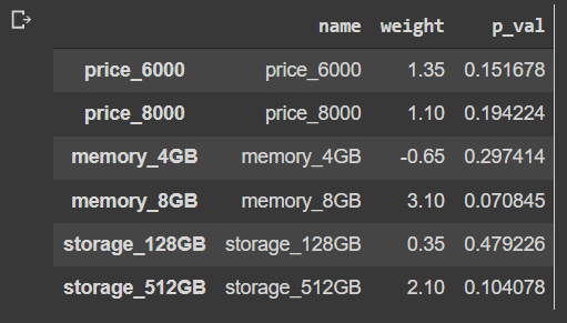
Figure 4.7: Product features’ weights and p-values

Although it’s important to consider the p-value to establish a level of statistical certainty, the model should be used with all variables. Here, we can use the Prob (F-statistic), which in our case is higher than 0.05, thus we cannot reject the null hypothesis. By looking also at a very high R-squared value, we can see that the model is overfitting. We would need to have much more data in order to create a significant model, but I’ll leave that challenge to you.

The next screenshot shows the characteristics of the product ordered by relative weight. In this case, users positively weigh the 8 GB memory, followed by the 128 GB storage:

sns.set()
xbar = np.arange(len(data_res['weight']))
plt.barh(xbar, data_res['weight'])
plt.yticks(xbar, labels=data_res['name'])
plt.xlabel('weight')
plt.show()

This results in the following output:

Figure 4.8: Product features’ weights sorted

It can be seen that memory has the highest contribution to evaluation, followed by storage.

We have seen how OLS can be used as a mean to estimate the importance of each product feature. In this case, it has been modeled as a regression over a single variable, but we could include information about the type of respondent in order to discover how different customer segments react to product features.

In the next section, we evaluate a case of a consumer goods product with even more features.

Working with more product features

In the example, we will use a dataset that contains many more features than the previous example. In this case, we will simulate data obtained from a crisp retail vendor that has asked some of its customers to rank its products according to their level of preference:

1. The following block of code will read the dataset, which is a CSV file, and will prompt us with the result:

   # Load data

   conjoint_dat = pd.read_csv('/content/conjoint_data.csv')

   conjoint_dat

This results in the following output:

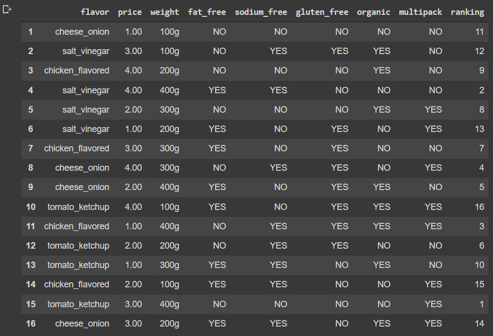
Figure 4.9: Crisps data

2. We can see that the data contains only categorical values, so it will be necessary to transform this categorical data into a one-hot vector representation using the get_dummies pandas function, which is what we do in the next block of code:

   conjoint_dat_dum = pd.get_dummies(conjoint_dat.iloc[:,:-1], columns = conjoint_dat.iloc[:,:-1].columns)

   conjoint_dat_dum

We can see that now we have created a set of columns that describe the product features using 1s and 0s:

Figure 4.10: Crisps data in a one-hot representation

3. We can now construct an OLS model using the one-hot vector representation of the product features and passing the ranking as the target variable:

   main_effects_model_fit = sm.OLS(conjoint_dat['ranking'].astype(int), sm.add_constant(conjoint_dat_dum))

   result = main_effects_model_fit.fit()

   result.summary()

This results in the following output:

Figure 4.11: OLS regression results

The terms AIC and BIC in the model summary, which stand for Akaike’s Information Criteria and Bayesian Information Criteria, respectively, are frequently used in model selection criteria; however, they are not interchangeable. BIC is a type of model selection among a class of parametric models with variable numbers of parameters, whereas AIC may be thought of as a measure of the goodness of fit of an estimated statistical model. The penalty for additional parameters is greater in BIC than in AIC. BIC penalizes free parameters more severely than AIC.

AIC typically looks for undiscovered models with high-dimensional reality. This indicates that AIC models are not accurate models. BIC, on the other hand, only encounters True models. Additionally, BIC is consistent, although AIC is not, it might be said. BIC will indicate the risk that it would underfit, while AIC is more suited to examine whether the model has anger that it would outfit. Although BIC is more forgiving than AIC, it becomes less forgiving as the number increases. Cross-validation can be made asymptotically equal with the help of AIC. BIC, on the other hand, is useful for accurate estimation.

The penalty for additional parameters is higher in BIC than in AIC when comparing the two. AIC often looks for an unidentified model with a high-dimensional reality. BIC, on the other hand, exclusively finds True models. AIC is not consistent, whereas BIC is. Although BIC is more forgiving than AIC, it becomes less forgiving as the number increases. BIC penalizes free parameters more severely than AIC.

4. The next code will create a DataFrame where we can store the most important values from the analysis, which in this case are the weights and p-values:

   data_res = pd.DataFrame({'name': result.params.keys(),

                            'weight': result.params.values,

                            'p_val': result.pvalues})

   data_res = data_res[1:]

   data_res

This results in the following output:

Figure 4.12: OLS variable weights and p-values

5. Now that we have the values arranged, we can check the significance of each one of the relationships to check the validity of the assumption and visualize the weights:

   xbar = np.arange(len(data_res['weight']))

   plt.barh(xbar, data_res['weight'])

   plt.yticks(xbar, labels=data_res['name'])

   plt.xlabel('weight')

   plt.show()

This results in the following output

:

Figure 4.13: Variable weights sorted by importance

In this case, it can be seen that there are factors that are positively related, such as the weight of 100 grams, and the option for the product to be fat-free, while there are other factors that are negatively related, such as the weight of 400 grams, followed by that the product is not fat-free.

One of the questions that might arise is this: If we have a regressor model to estimate the product score, can we use the same model to predict how customers will react to new product combinations? In theory, we could, but in that case, we would have to use a scoring system instead of a ranking and have much, much more data. For demonstration purposes, we will continue regardless as this data is difficult to get and even more difficult to disclose.

Predicting new feature combinations

Now that we have properly trained our predictor, we can use it besides capturing information about the product features’ importance to also provide us with information about how new product features will perform:

1. After going through the EDA, we will develop some predictive models and compare them. We will use the DataFrame where we had created dummy variables, scaling all the variables to a range of 0 to 1:

   from sklearn.preprocessing import StandardScaler

   X = conjoint_dat_dum

   y = conjoint_dat['ranking'].astype(int)

   # The target variable will be normalized from a ranking to a 1 to 10 score

   y = y.apply(lambda x: int(x/len(y)*10))

   features = X.columns.values

   scaler = StandardScaler()

   scaler.fit(X)

   X = pd.DataFrame(scaler.transform(X))

   X.columns = features

This results in the following output:

Figure 4.14: Scaled variables

One of the most popular ML models is Logistic Regression, which is an algorithm that uses independent variables to make predictions. This algorithm can be used in the context of classification and regression tasks. It’s a supervised algorithm that requirs the data to be labeled. This algorithm uses example answers to fit the model to the target variable, which in our case is the product ranking. In mathematical terms, the model seeks to predict Y given a set of independent X variables. Logistic Regression can be defined between binary and multinomial logistic regression. Namely, the characteristic of these two can be described as follows:

• Binary: The most used of all the types of logistic regression, the algorithm seeks to differentiate between 0s and 1s, a task that is regarded as classification.
• Multinomial: When the target or independent variable has three or more potential values, multinomial logistic regression is used. For instance, using features of chest X-rays can indicate one of three probable outcomes (absence of disease, pneumonia, or fibrosis). The example, in this case, is ranked according to features into one of three possible outcomes using multinomial logistic regression. Of course, the target variable can have more than three possible values.
• Ordinal logistic regression: If the target variable is ordinal in nature, ordinal logistic regression is utilized. Each category has a quantitative meaning and is considerably ordered in this type. Additionally, the target variable contains more categories than just two. Exam results, for instance, are categorized and sorted according to quantitative criteria. Grades can be A, B, or C, to put it simply.

2. The primary distinction between linear and logistic regression is that whereas logistic regression is used to solve classification problems, linear regression is used to address regression difficulties. Target variables in regression issues might have continuous values, such as a product’s price or a participant’s age, while classification problems are concerned with predicting target variables that can only have discrete values, such as determining a person’s gender or whether a tumor is malignant or benign:

   # Logistic Regression

   from sklearn.model_selection import train_test_split

   from sklearn.linear_model import LogisticRegression

   from sklearn import metrics

   X_train, X_test, y_train, y_test = train_test_split(X, y, test_size=0.5, random_state=101)

   # Running logistic regression model

   model = LogisticRegression()

   result = model.fit(X_train, y_train)

By feeding the train set features and their matching target class values to the model, it can be trained. This will help the model learn how to categorize new cases. It is crucial to assess the model’s performance on instances that have not yet been encountered because it will only be helpful if it can accurately classify examples that are not part of the training set.

The average of the error squares is measured by the mean squared error (MSE), which is the average of the sums of the squares of each discrepancy between the estimated value and the true value.

3. The MSE is always positive, although it can be 0 if the predictions are completely accurate. It includes the variance of the estimator (how widespread the estimates are) and the bias (how different the estimated values are from their actual values):

   prediction_test = model.predict(X_test)

   # Print the prediction accuracy

   print(metrics.mean_squared_error(y_test, prediction_test))

This results in the following output:

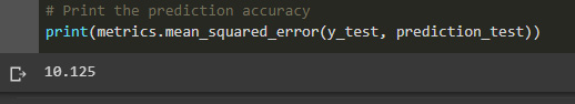
Figure 4.15: MSE of the simple regression

4. The MSE is always 0 or positive. If the MSE is large, this indicates that the linear regression model does not accurately predict the model. The important point is that MSE is sensitive to outliers. This is because the error at each data point is averaged. Therefore, if the outlier error is large, the MSE will be amplified. There is no “target” value for MSE. However, MSE is a good indicator of how well your model fits your data. You can also indicate whether you prefer one model to another:

   # To get the weights of all the variables

   weights = pd.Series(model.coef_[0],

                    index=X.columns.values)

   print(weights.sort_values(ascending = False)[:10].plot(kind='bar'))

This results in the following output:

Figure 4.16: Linear regression top variable contribution

Here, we can see the first 10 variables that the model has identified as positively related to the score.

5. The next code will show us the ones that are more negatively related:

   print(weights.sort_values(ascending = False)[-10:].plot(kind='bar'))

This results in the following output:

Figure 4.17: Linear regression negative variable contribution

Random Forest is a supervised learning (SL) algorithm. It can be used both for classification and regression. Additionally, it is the most adaptable and user-friendly algorithm. There are trees in a forest. A forest is supposed to be stronger the more trees it has. On randomly chosen data samples, random forests generate decision trees, obtain a prediction from each tree, and then vote for the best option. They also offer a fairly accurate indication of the significance of the feature.

Applications for random forests include feature selection, picture classification, and recommendation engines. They can be used to categorize dependable loan candidates, spot fraud, and forecast sickness.

A random forest is a meta-estimator that employs the mean to increase predicted accuracy and reduce overfitting. It fits a number of decision-tree classifications over various dataset subsamples. If bootstrap = True (the default), the size of the subsample is specified by the max_samples argument; otherwise, each tree is constructed using the complete dataset. In random forests, each tree in the ensemble is constructed using a sample taken from the training set using a substitution (that is, a bootstrap sample). Additionally, the optimal split of all input features or any subset of max_features size is discovered when splitting each node during tree construction.

These two random sources are used to lower the forest estimator’s variance. In actuality, individual decision trees frequently overfit and have considerable variance. Decision trees with partially dissociated prediction errors are produced when randomness is added into forests. The average of these projections can help certain inaccuracies disappear. By merging various trees, random forests reduce variation, sometimes at the expense of a modest increase in distortion. The variance reduction is frequently large in practice, which leads to a stronger overall model.

Instead of having each classifier select a single class, the scikit-learn implementation combines classifiers by averaging their probabilistic predictions:

from sklearn.ensemble import RandomForestClassifier
model_rf = RandomForestClassifier(n_estimators=1000 , oob_score = True, n_jobs = -1,random_state =50, max_features = "auto",max_leaf_nodes = 30)
model_rf.fit(X_train, y_train)
# Make predictions
prediction_test = model_rf.predict(X_test)
print(metrics.mean_squared_error(y_test, prediction_test))

This results in the following output:

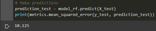
Figure 4.18: Random Forest MSE

One of the available options in terms of ML models is the Random Forest algorithm, which is implemented in the scikit-learn package and includes the RandomForestRegressor and RandomForestClassifier classes. These classes can be fitted to data, yielding a model that can then be used to create new predictions or to obtain information about feature importance, a property that is at the core of the importance of conjoint analysis, as in the following example:

importances = model_rf.feature_importances_
weights = pd.Series(importances, index=X.columns.values)
weights.sort_values()[-10:].plot(kind = 'barh')

This results in the following output:

Figure 4.19: Random Forest variable importance

The XGBoost library is a highly effective, adaptable, and portable library for distributed gradient augmentation. It applies ML techniques within the Gradient Boosting framework and offers parallel tree amplification (also known as GBDT and GBM), which gives quick and accurate answers to a variety of data science issues. The same code can handle problems that involve more than a trillion examples and runs in massively distributed contexts.

It has been the primary impetus behind algorithms that have recently won significant ML competitions. It routinely surpasses all other algorithms for SL tasks due to its unrivaled speed and performance.

The primary algorithm can operate on clusters of GPUs or even on a network of PCs because the library is parallelizable. This makes it possible to train on hundreds of millions of training instances and solve ML tasks with great performance.

After winning a significant physics competition, it was rapidly embraced by the ML community despite being originally built in C++:

from xgboost import XGBClassifier
model = XGBClassifier()
model.fit(X_train, y_train)
preds = model.predict(X_test)
metrics.mean_squared_error(y_test, preds)

This results in the following output:

Figure 4.20: Random Forest MSE

We can see that the MSE for the random forest is even greater than the linear regression. This is possible because of the lack of enough data to be able to achieve a better score, so in the next steps, we would have to consider increasing the number of data points for the analysis.

Summary

In this chapter, we have learned how to perform conjoint analysis, which is a statistical tool that allows us to undercover consumer preferences that otherwise would be difficult to determine. The way in which we performed the analysis was by using OLS to estimate the performance of different combinations of features and try to isolate the impact of each one of the possible configurations in the overall perception of the client to undercover where the consumer perceives the value.

This has allowed us to create an overview of the factors that drive users to buy a product, and even be able to predict how a new combination of features will perform by using ML algorithms.

In the next chapter, we will learn how to adjust the price of items by studying the relationship between price variation and the number of quantities sold using price elasticity.