
Mathias Verraes’ joke about two hard problems in distributed systems is based on a saying by Phil Karlton formerly of Netscape. He quipped “There are only two hard things in Computer Science: cache invalidation and naming things.”
I am notoriously bad at naming things (as you have no doubt discovered in earlier chapters). However, I have a rock solid solution to cache invalidation. Query inverses determine not only which caches should be invalidated but also precisely how they should be updated.
When we think of caching, we often think of improving performance or scalability. But the most important cache is the one that the user is looking at. User interfaces are caches of query results stored temporarily in view models and browser DOMs. When that cache is invalidated, the user expects their view to automatically update. Failure to update the UI leads to a frustrating user experience. The browser’s F5 button and “pull to refresh” are interface metaphors that admit defeat.
On the face of it, you would expect caching of immutable data to be easy. If data doesn’t change, the cache is always up-to-date. The point of the cache, however, is not to store a copy of the immutable facts. It’s to store a copy of query results. It is query results—not raw facts—that appear on a user interface. And so we must find a strategy for determining when a query’s results have been affected.
- 1.
Which caches or UI components are invalidated?
- 2.
What results should be added to or removed from those caches and components?
Query inversion answers one—and sometimes both—of those questions. The views that are affected can always be found by traversing the query from the introduced fact backward. The results to add or remove can usually be given by the tail of the query from the introduced fact forward. And even when the inverse does not answer the second question, then we simply need to rerun the query to bring the view up-to-date.
Mechanizing the Problem
Determining what to update when certain events take place is the bread and butter of application development. We do it intuitively all the time. Whether responding to user-input events, API commands, or messages in a queue, a developer decides what state is out-of-date. It might be a view model that needs to raise property changed events or an array of results that needs to be flushed and reconstructed. Developers make those decisions.
Intuition, however, fails in two important ways. First, it is easy to miss dependent state that needs to be updated. And second, update logic needs to be revisited as requirements are added. For the first problem, we simply test until we think we’ve found all of the reasons for a view to change. And for the second problem, we analyze each new feature for how they interact with existing behaviors. We add these as acceptance criteria, modify all affected areas of code, and test for regressions. Because of this, new changes take longer to make and have a greater chance of introducing bugs.
A better solution is to remove cache invalidation and UI update decisions from developer’s hands. If the system could decide which caches to rebuild and which user interface components to update all on its own, then that logic would not clutter the code. The decisions can be made mechanically without the risk of human error. And they can be updated automatically as the system grows, keeping each new feature as quick and safe to add as the first one.
The good news is that the system already has enough information to make cache invalidation decisions. Every cache and user interface component is initially populated with a query. That query describes a path through the system’s data that yield the results to store or render. By processing the query when it is first executed, the system can determine what new facts will affect the results in the future. All we need to do is invert the query and begin watching for those new facts.
Let’s begin by finding a formal vocabulary for describing queries. This will help us not only to execute them but to mechanically invert them.
The Anatomy of a Query
A query written in the Factual Modeling Language describes the types and relationships among facts. It gives the conditions under which certain facts should be included. A Factual query is a declarative statement of the results that we seek. This description needs to be translated into something actionable.

The query visualized as a path over the fact graph
The dotted arrows indicate the path along which the instance graph will be traversed. It describes how we will execute the query. We can formalize that process as a pipeline. This will be used not only for executing queries but also for computing their inverses.
A Sequence of Steps
A query is a sequence of steps . Each step moves from one fact type to another along an edge. The edge is the predecessor/successor relationship between the two facts. Each edge has a role: the name given to the predecessor within the successor’s type definition. So we can define a step between facts of type A and B as going up to the predecessor or down to the successor along an edge with a given role.

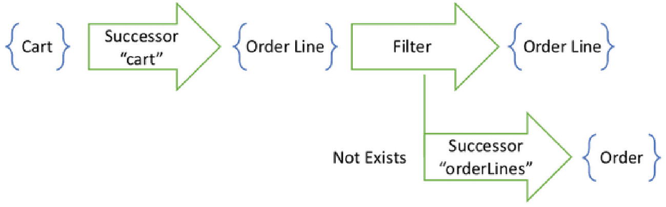
The first step in the pipeline takes a set of carts to a set of order lines
A query is a path from one fact type A to another fact type Z. We will build a pipeline of components, each one taking a set of input facts and producing a set of output facts. The initial set contains only one fact: the starting point of the query.
Filter by Existential Condition
Some components within the pipeline will not be steps at all. They will not move up to a predecessor or down to a successor along an edge. Instead, they will filter the incoming set. Filters are given as a Boolean expression of existential conditions. Each condition’s quantifier is either exists or not exists. The body of the condition is another query, which starts at the fact type where the filter is applied.

The second step filters order lines based on a subquery
A pipeline composed of three operations
These are the components that we will manipulate to compute the inverse of the query. And it starts by computing the affected set. To understand how to do that, let’s return to our familiar zigzag paths.
The Affected Set
The first question that a query inverse answers is which caches and views are affected by a new fact. It identifies those caches and views by the starting point from which the query was first executed.
Every query has a starting point. Any particular cache or user interface component holds the results of a query for a specific starting fact. Different users will be running the same queries, but each will start at a different fact. Hence their caches will be different. As they navigate through the user interface, they will render components by running queries. While many of these components will run the same query, each one will start from a different fact. The starting point of a query determines which user interface component to update, or which cache to invalidate.
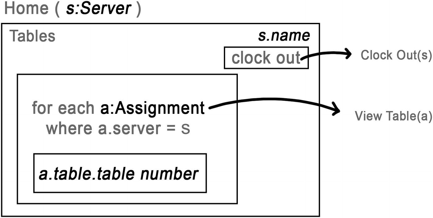
The user interface component showing assigned tables starts at the server fact
Computing the Affected Set
When the table list view first loads, it runs the query shown in the wireframe. That query determines which tables to show in the list. But that query also provides all of the information needed to compute the affected set of any subsequent Assignment. That is the role of the inverse.

The query for a server's table assignments is a single step to its successor

The inverse query simply follows the same step in the opposite direction
Inverting Longer Queries
The preceding example is extremely simple. It demonstrates the process of query inversion, but does not reveal any of the nuance. When we start to examine longer queries, we find that we have a few more considerations.
A query with only a single step can only be affected by one kind of introduced fact. It has only one inverse. But a query with multiple steps can be affected if any of them is introduced. Longer queries have more inverses. So the process of query inversion is not simply reversing the chain of steps. It is producing all reversed chains that point back to the starting point.

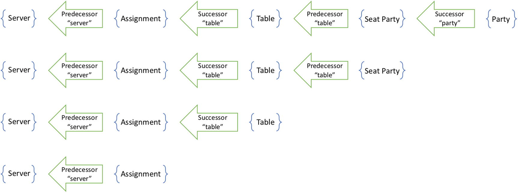
A query of four steps yields all parties seated at a table assigned to a server

When a SeatParty fact is introduced, all servers assigned to the table are affected
Each of the inverses is a query from a different fact type back to a Server. All told, this query has four inverses. They start at each of the types Assignment, Table, SeatParty, and Party. They get progressively longer as they all terminate at the server.
Unsatisfiable Inverses
A query inverse is executed when a new fact is introduced. This could be the result of a user action. Or it could be that the new fact arrived from some other device. In either case, the fact that was introduced was not present before and is therefore not represented in the query results. That is, after all, the very reason that we are updating the view.
Knowing that the new fact has just arrived at this node tells us something quite useful. It assures us that the fact currently has no successors.
For a fact to have successors, it must have been introduced before the successors were. A user can only take actions that reference existing facts. And for a peer device to share a fact with this node, it must have first shared all of its predecessors. Said more formally, facts are introduced in topological order.
Because the fact that was just introduced does not yet have any successors in the system, we can be assured that any queries that start with a successor step will yield no results. In particular, any of the inverses that begin by stepping down to a successor will necessarily yield an empty affected set. Such inverses are unsatisfiable. They will never find a view that needs to be updated. They can therefore be ignored.

When a new table is introduced, the query for affected servers begins with a successor step
Considering this optimization visually, observe the original query as a zigzagging path through the graph. It has hills and valleys as it goes up to successors and down to predecessors. This optimization tells us that we only need to consider inverses that start in valleys. If an inverse starts on a hill, then the first step of the inverse query is down to a successor. Of the four inverses that we computed from the original query, only two are satisfiable : the ones starting from the Assignment and from the SeatParty.
Walking Backward

A pipeline from a set of servers to a set of parties that they take care of
The four inverses of the original query have the opposite steps

Only two of the inverses are satisfiable
To render the party list, we execute the original pipeline starting from the Server. Then, whenever a new SeatParty fact is introduced, we execute the first inverse pipeline in Figure 9-13 to find the affected views. And, whenever a new Assignment fact is introduced, we execute the second inverse pipeline. There are no other events that could affect the view. This mechanical process finds all ways in which the view could be affected.
Proof of Completeness
The claim that there are no other events that could affect the view needs to be defended. It is by no means obvious. Let’s take a moment to do so before we proceed.
To begin, we need to define what we mean by “event.” An event could be something that the user themselves has done on this node, or it could be information that arrived from some other node. If it happened on this node, it could either be a transient action such as navigation or a permanent action such as saving a new fact. Transient actions will lead to new starting points for queries and will therefore replace old views with new ones. Permanent actions are always analyzed as introductions of new facts. Our analytical tool of Historical Modeling allows no other permanent actions, such as modifications or deletions.
So every event that could affect an existing view would therefore be the introduction of a fact. This might be one that the user introduced themselves or one that arrived from a peer node. In either case, if we were to rerun the query of an affected view, that new fact would have some potential effect on the results.
Our assertion of completeness is equivalent to saying that the inverses find all starting points that could be affected by the introduced fact. To convince ourselves that this is true, we examine the sets of facts that appear along the pipeline. If a fact appears in one of those sets, then it potentially has an effect on the pipeline’s results. If it does not, then it could not have an effect.
Observe that the reverse of a predecessor or successor step yields a superset of the original starting set. If we start from one set of facts and find all successors in a given role, we are picking out all edges by role and predecessor. Going in the opposite direction, we are picking from among the same edges, but now by role and successor. The edges that produced a result in the original step will be among those included in the reverse step. And so the reverse of a predecessor or successor step will yield all starting facts that could possibly contain a given destination fact.
So far this proof only considers predecessor and successor steps. We will complete the proof by considering filters after we examine existential conditions.
New Results
Knowing which view to update is a great start. Once we know that a view is affected, we can just run its query again from its starting point to find the new state. But we can often do better. Sometimes, the query inverse tells us exactly what new results should be added to the view.

The remainder of the query (shown after the dot) gives the new results to add to the affected view
To execute these inverses, start with an introduced fact. Execute the reverse pipeline to find the affected set. Then execute the forward pipeline to find the new results.
When a party is seated, for example, a new SeatParty fact is introduced. Query for all servers assigned to the table at which the party was seated. To each of their views, add the party. And when a new table assignment is introduced, follow the pipeline backward to the affected server. Update that server’s view with all parties currently seated at that table.
Your intuition may have led you to write exactly this code. You might have realized that you don’t need to rerun the whole query to update the view. But following a mechanical process to automatically produce the optimal algorithm, you now have confidence that no edge cases were missed and no new features will break this code.
Forward Optimization
As before , we know that the introduced fact has no successors. Just as we used this observation to remove unsatisfiable inverses, we can also identify unsatisfiable results. If the forward query begins with a successor join, then the entire inverse can be eliminated. We might be able to find some affected views, but we know that this new fact will introduce no new results.

Some queries might take several successor steps in a row
Computing the inverse at every point along the path, we find that the reverse pipeline from C starts with a predecessor step. It might at first appear satisfiable. However, observe that the forward pipeline from C to D begins with a successor step. This inverse is therefore not satisfiable. Only the inverse starting at D yields new results for an affected view. Inverses always start from the valleys of the fact type graph.
Existential Conditions
So far we’ve examined simple queries. They are a sequence of steps, each toward a predecessor or successor. However, most queries used to populate a user interface or seed a cache are more complex. They are composed not just of predecessor and successor steps but also of exists and not exists conditions. Let’s add these operators to our basic inverses and see how they evolve.

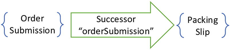
A pipeline having an exists condition
Once we have this pipeline, we can execute the query. The set of OrderSubmissions leaving the filter component will be a subset of those entering. Each of the order submissions is fed into the successor step, and only those that produce a result are kept. Consider, then, what happens to the results when a new PackingSlip is introduced. If it brings the number of subquery results from 0 to 1, then it causes its parent OrderSubmission to appear in the results.
Recursive Inversion
The entry point of a subquery is the type on which the filter operates
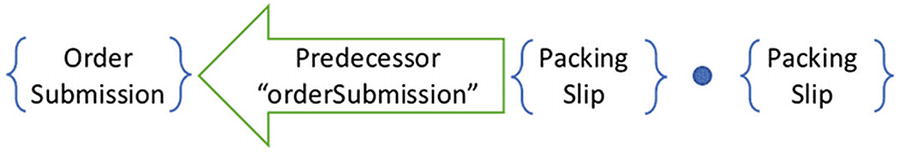
The inverse of the subquery adds the introduced packing slip to the affected order submission
Popping the stack and returning to the upper portion, we reason that introducing a PackingSlip causes the introduction of an OrderSubmission . We arrive at this conclusion based on the exists quantifier. An order submission without a subsequent packing slip would be filtered out. So introducing the packing slip adds it into the pipeline.
We can pop the stack and continue analyzing the pipeline as if it was the OrderSubmission that was introduced instead of the PackingSlip . We could, that is, except for one small caveat. Since the OrderSubmission was already known to this node, it might possibly have other successors. We therefore cannot apply the valley optimization that we used previously. We must retain the inverse even if the existential condition does not appear in the valley of the graph. The valley optimization only applies to the innermost subquery.

The inverse starts with the inverse of the subquery and continues as if the affected fact was introduced
Tail Conditions
In the preceding example, we don’t care about the packing slip that was added to the subquery results. All we cared about was the fact that results were added. The inverse of the subquery shown in Figure 9-18 shows the added pipeline after the dot. But we dropped that detail as unimportant in Figure 9-19.
In general, however, that detail matters. The subquery tells us which filter condition might be affected by the introduced fact. It does not, however, guarantee us that the condition is indeed true. To have this guarantee, we need to know that the introduced fact resulted in some actual additions. This is why we will in general want to execute the tail of the subquery. The affected filter condition is only guaranteed to be true if the tail yields some results.
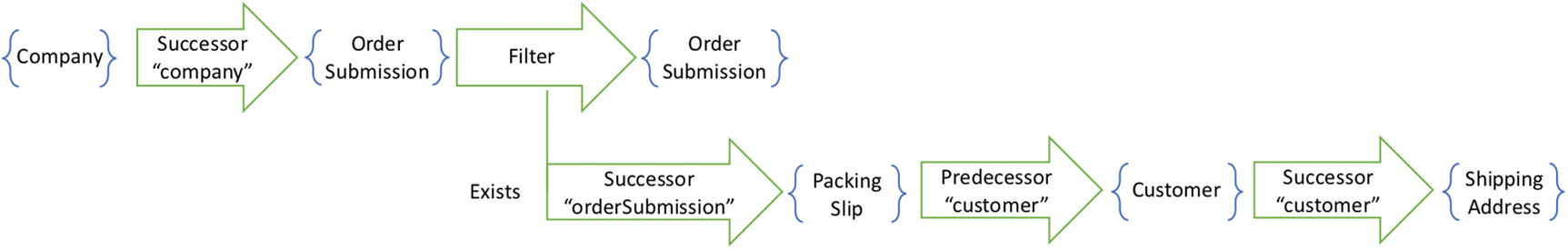
The revised pipeline has two extra steps in the subquery

The inverse of the subquery retains the two new steps in its tail
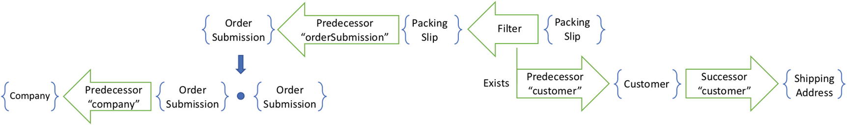
The tail of the subquery becomes a condition of a filter
In general, we must always include the tail of an exists subquery inverse as a filter condition. In some cases, that filter condition turns out to be a tautology. It will always be satisfied, as in the example featuring a trivial tail pipeline. When the condition is a tautology, the filter can be optimized away.
Removing Results
The exists clause was the simpler of the two existential quantifiers. It only has the effect of introducing new results. The other clause—not exists—allows a new possibility. This clause can remove results. The consequences are far more significant than simply negating a condition.

A not exists clause filters based on a subquery
The inverse of a not exists clause causes the removal of results in the outer pipeline
When Removal Isn’t Removal
An inverse that removes results is significantly different from an inverse that adds them. It’s not just a matter of reversing a sign. The difference is in what we can guarantee. We cannot always know that the result that the inverse wants us to remove should truly be removed. It is much more difficult to prove a negative.
When a result is added to an affected query, we can guarantee that the new result would actually be returned were we to run the query again. We would like to make a similar claim about removed results. We would like to assert that removed results would not be returned from the query. Unfortunately, this is not always possible.
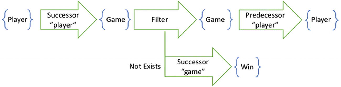
A pipeline for finding current opponents takes an additional predecessor step to the player
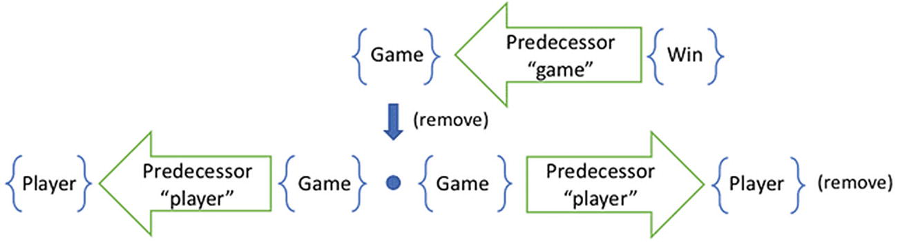
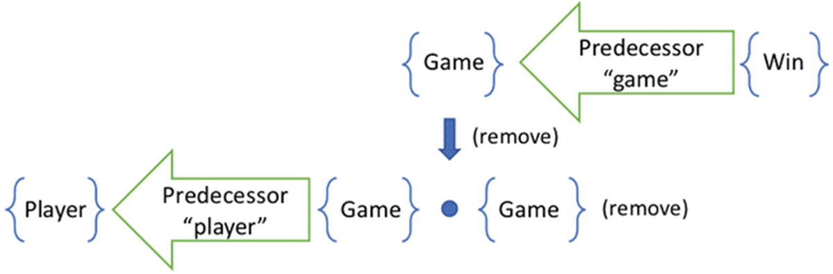
The inverse removes the player of the removed game
This additional step would have us remove the opponent of a game that just ended. When the Win is introduced, the Game cascades down and removes the opponent from the affected view. However, it is possible that another game with this same opponent is in progress. There is more than one way to traverse the graph to get to this opponent. Removing one of these paths does not guarantee that no other paths exist.
The previous query was safe. We could guarantee that any game will be removed from the cache when a successive win was introduced. No matter how we traversed the graph, the filter was applied to the game itself. But if the pipeline extends beyond the filter, then we can no longer make that guarantee. If the remove set is a nontrivial pipeline, then we have to check all possible paths.
In situations like this, a removal cannot guarantee that the removed result is not still a valid result by some other path. As a consequence, we must run the original query again. The affected set tells us which caches to invalidate. But the remove set does not tell us which results to remove. At best, it gives us a set of candidates that we can check.
Nested Subqueries
As we process nested subqueries, we will need to keep track of whether they add or remove results. It is not uncommon for a not exists subquery to have a not exist subquery of its own. When this occurs, introducing a fact to the innermost subquery will add a result to the view. Each recursive descent into a not exists subquery flips the direction of the effect.

The restore pattern yields a pipeline with nested not exists filters
To find the inverses of this query, we traverse the pipeline recursively. After descending two levels, we invert the innermost query. This tells us that introducing an EntityRestore fact affects the predecessor EntityDeletion. It has the effect of removing that EntityDeletion . This is an effect that we can guarantee, since we have inverted a not exists clause and can prove that the successor exists.
Popping the stack, we then determine the effect of removing the EntityDeletion . The inverse tells us the affected set of Entity facts. Removing the entity deletion would ideally have the effect of adding the entity. However, this is not an effect we can guarantee.
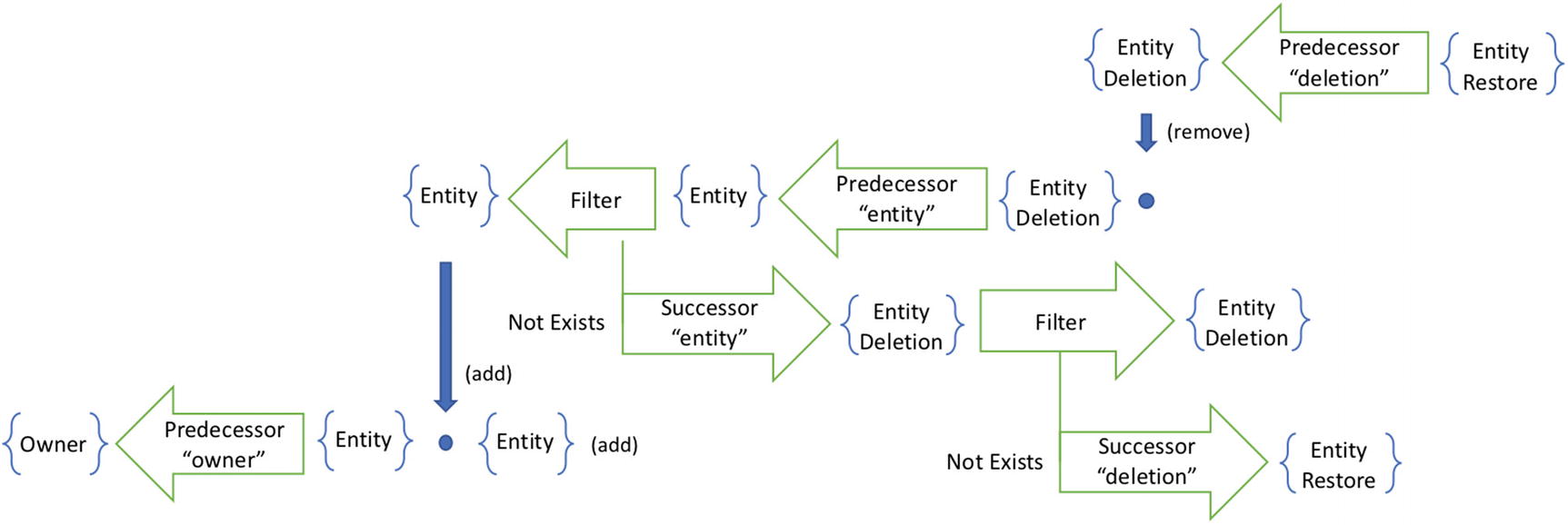
In inverse of two nested not exists clauses is a pipeline that causes the addition of facts
In general, we can guarantee the effect of an inverse based on adding a fact. The innermost subquery is always of this form, as it captures the introduction of a new fact. But any inverse based on removing a fact cannot be guaranteed. There may be other paths through the graph that keep the condition as it is. Therefore, we must always append a filter testing the original condition to the inverse.
Tautological Conditions
In the previous examples of inverses, I left off an important detail. The inverse must preserve the existential condition of the original query. I left it off both for clarity and because I chose examples in which it didn’t matter. In each of the previous examples, the existential condition is guaranteed to be true under the circumstances in which it was applied. A logical predicate that is always true is called a tautology. When we recognize tautologies within inverses, we can optimize them away.

A query with a compound condition defines a pipeline with two subqueries
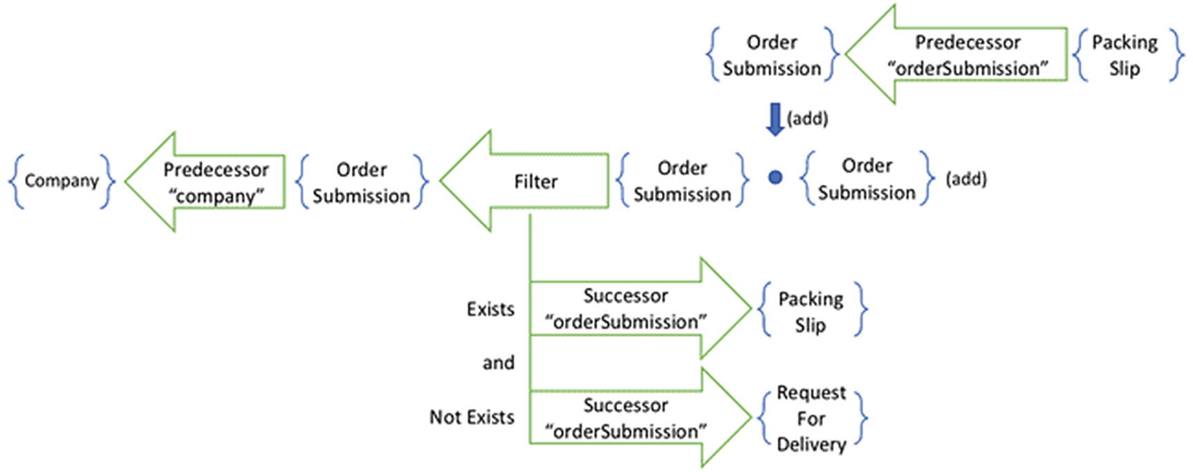
The inverse pipeline retains the existential conditions of the original query

We can eliminate tautological conditions from a filter
The pipeline gives us no knowledge about the remaining condition. We must still, therefore, verify it before we add the resulting order submission. The first time that we examined this inverse, the RequestForDelivery clause was not in the pipeline. We therefore ended up with a filter having only a tautological condition. We optimized away the filter, as it would have no effect.
The resulting inverse implies a procedure. When a packing slip is introduced, add the order submission to the cached results, but only if it is not drop-shipped. As a human analyst, one might ask “why would we create a packing slip for a drop-shipped order?” Doing so would be absurd. This observation might lead a human designer to eliminate this check. But a mechanical inverter has no such bias. It will produce code that is logically correct even if it makes no business sense. And as a result, it will work correctly in nonsensical edge cases where a solution based upon intuition would fail.
In general, we will find two scenarios by which a condition is a tautology. First, we will have exists clauses seeking facts that were just introduced. And second, we will have not exists clauses seeking successors of newly introduced facts. The one we just examined is an example of the first. The second is an extension of the valley optimization. We eliminated inverses that began outside of a valley. Those inverses began with successor steps, either in their affected set or their new results. By the same token, we can consider any not exists clauses at the very head of the inverse beginning with a successor step to be a tautology.
When we reverse the not on the two general cases mentioned earlier, we find a different optimization. The opposite of a tautological predicate is an unsatisfiable predicate. It is possible that an inverse will contain a not exists clause seeking introduced facts. Given that the inverse fires only when those facts are introduced, we know these conditions to be false. It is also possible that an inverse will contain an exists clause for successors of introduced facts. Again, since these facts were newly introduced, these conditions must be false. Unsatisfiable conditions within an or statement can be eliminated; those within an and statement make the whole statement unsatisfiable. A mechanical query inverter will optimize away these statements as well and even optimize away the entire inverse if the filter condition is deemed unsatisfiable.
Proof of Completeness Continued
Now that we have a better understanding of the effect of filters on the query inverse, we can finish the proof of completeness. We’ve already shown that an inverse made up only of successor and predecessor steps does not exclude any possible affected starting points. We will now show the same for inverses containing filters.
A predecessor or successor step has the property that the inverse produces a superset of the original starting set. We relied on this to show that all starting points that would include the introduced fact would be in this superset. Filter components do not have this property. A filter in either direction yields a subset of the starting set. For filters, we must consider whether we are adding or removing a fact.
If we are adding a fact—such as for the innermost subquery responding to the introduced fact—then we can assert that the added fact would only have an effect on the query if it passed through the filter in the original pipeline. If it was filtered out, then it would have no downstream effect. Therefore, applying the filter in the opposite direction, even though it produces a subset, produces precisely the subset that would truly be affected.
If we are removing a fact, on the other hand, this logic does not hold. We are seeking an affected set of starting points whose pipelines used to contain the removed fact, but no longer do. Therefore, a filter would exclude precisely the starting points that would be affected by the removed fact. Reversing the filter does not solve the problem. The affected set could be filtered for more than one reason, and any of the remaining filters might incorrectly exclude it.
The solution, then, is to remove any filters from the affected set of remove inverses. The only filter that these inverses should have is the one at the end that verifies that the filter condition is indeed false for these affected starting points. Any other filter would reduce the affected set and potentially miss effects.
Potential vs. Actual Change
When reasoning through the effect of existential conditions, we made an assumption. We assumed that the effect of a subquery inverse would always be to change the filter condition from false to true and thus add the result or from true to false and thus remove it. Now that all of the complexity of subquery inverses, tautologies, and unsatisfiable predicates are on the table, we can acknowledge that that assumption is not in fact true. Once we do so, we can then see what simple extra step we need to take to defend against those cases where it is false.
We first introduced the assumption while examining the exists clause. There, we said that if the introduced fact brings the number of subquery results from 0 to 1, then the condition becomes true, and new results are added. We then proceeded to find inverses of the subquery, which we can safely assert will increase the number of subquery results. However, we had no evidence that they brought the number of results from 0 to 1. If the subquery already had results, then this new one would have no appreciable effect. The filter condition is already satisfied.
By continuing as if the new fact brought the number of subquery results from 0 to 1, we made the assumption that the new results it adds were not already results of the original query. Because this assumption is false, we might find ourselves adding results to a cache or view that are already present. And so, the consequence of making this assumption for an exists clause is duplication.
Removing Absent Results
A similar assumption arose unstated while we examined the not exists clause. Here, we proceeded to evaluate inverses of the condition under the assumption that any new fact would bring the number of results from 0 to 1. When viewed through the not exists clause, this would change the filter condition from true to false and therefore remove results. But if the subquery already had results, one more would not make the filter condition any more false. The effect of running an inverse in these circumstances would be to attempt to remove a result that was not in the cache.
There is an easy solution to this problem, and a hard one. Let me first describe the hard one, as it is interesting, but ultimately pointless. Because the graph of facts is immutable, introducing a new fact does not destroy information. We still have the capability of seeing the graph as it was before the fact was introduced. We could therefore compute the filter condition as it was just before the introduction of the fact that triggered the inverse.
If we run the filter condition—whether an exists or not exists clause—while ignoring the new fact, we can see if it used to be false. If so, we know that the introduction of the new fact was precisely what made it true. We would know that the subquery set changed from 0 to 1, and therefore the effect is real.
This solution is interesting because it is a specific example of a powerful analysis technique. It demonstrates that we can answer hypothetical “what if” questions by running queries while ignoring subsets of the directed acyclic graph. These questions can provide insights as to how the system appears on different nodes. They give us a powerful “time travel debugging” capability popularized by frameworks like Elm and Redux. But alas, for solving the problems of cache duplication and removing absent results, there is a much simpler solution.
Caches Are Sets
The results of a Factual query are always sets. They do not impose an order, and they do not permit duplicates. Therefore, any cache or view seeded by a query will have at its core a set. It might further apply an order on top of that set or project the set through some aggregate function, but what it started with was an unordered set of distinct facts.
As long as a cache or view retains the set of facts, it can easily protect against the assumption that every potential change is an actual change. If an inverse reports that an introduced fact adds a set of results, the cache simply performs the set union. It ignores any results that are already in the set. It only adds the ones that are truly new. Similarly, to process an inverse that removes results, the cache performs a set difference. It only removes results that were actually in the set to begin with.
It is tempting when creating a view to simply keep track of the projected DOM, XAML, or other visual elements. And if users of a cache are only interested in a mutable projection of some facts, not the raw immutable results themselves, then it stands to reason that the mutable projection is all that the cache needs to store. However, the simplest solution to the cache invalidation problem is to keep the set that leads to the projection. In response to a query inverse, perform a set union or difference. And then project the part that has changed.
Query Inversion in Practice
As you’ve just witnessed, query inversion is a complicated business. There are several edge cases, scenarios, and optimizations to consider. Fortunately, the process can be automated. Developers need not compute the inverse of a query by hand.
The mechanical process of query inversion is guaranteed to produce an affected set that identifies all possible invalid caches. Furthermore, it often produces an add or remove set that describes exactly what set union or difference to compute. But even when the inverse is too complex to produce such exact instructions, running the query again will produce the correct results.
I have produced a couple of implementations of the query inversion algorithm in the past. The first was for an open source project called Correspondence. The second was for a more recent open source project called Jinaga. Both of these projects derived inverses from the developer’s original queries to determine which views to update as new facts are introduced. Their behavior was surprising to me, even knowing the math behind them. And I found that my confidence and productivity were greatly improved by having a query inverter working on my behalf.
Following publication of this book, I will maintain an open source reference implementation of the query inversion algorithm. With the help of readers, I may find edge cases and optimizations that I missed in this chapter. Those improvements will become part of the reference implementation. Any projects wishing to use query inversion can learn from that implementation and compare results as a form of automated testing. You may find a link to that reference implementation at the book’s website on Apress, at at immutablearchitecture.com.