
In the not too distant past, most programs ran on a single computer. After the proliferation of JavaScript in the web browser, apps on mobile phones, and microservices in the cloud, most programs that we write today run across many computers. Whereas distributed systems used to be a specialty, today they are the default. We need to update other defaults to meet that demand.
One of the defaults that we need to update is the assumption that data has a location. Some systems try to treat remote objects as if they are local. DCOM uses object identifiers to make a proxy look like a local instance of a remote object. Remote procedure calls (RPCs) try to hide the reality of network communication behind an interface that looks like a normal function. The problems with these systems have been well covered elsewhere, so I will not rehash them here.
The assumptions of locality that I want to examine are a bit more subtle. Even when we replace RPCs with messages, and object identifiers with URLs, it is easy to assume that data has a location. We make that assumption whenever we identify a “source of truth” or a “system of record.” We rely upon location whenever a single node generates unique identifiers. Our default mode of programming what happens at a machine leaks into the behaviors that we program into the system as a whole.
So many of the behaviors that we’ve come to expect from our systems depend upon location. We expect items to be sequentially ordered. We expect the system to reject duplicate names. We expect that when the user updates a property of an object, it will have the value that they just assigned. Indeed, the expectation that properties to even have single values is a location-dependent assumption.
A system that depends upon location will misbehave when that location becomes unavailable. If we strive instead for location independence, we will construct systems that are more responsive, resilient, and reliable. They can act autonomously without communicating with remote nodes. They can tolerate network failures without introducing defects. And the decisions that a user makes in isolation will be honored when other nodes and users learn of that decision.
Modeling with Immutability
At its core, the assumption of location is all about mutability. A variable is a place that stores a value. Programs use the variable to address that location and read its value. After the variable is updated, we expect the program to read the new value the next time it looks. Scale this up to the level of the distributed system, and you have location dependence. A system depends upon data being in a location specifically because that data is allowed to change.
If we search instead for a model of computing that is based on immutability, then dependence upon location fades away. If an object cannot change, then every copy of it is just as good. There is no need to know where the object is stored, where it was created, or which subsystem is the source of truth.
Of course, we need to model domains that change over time. So, the concepts of time and change need to be re-examined in the light of immutability.
Synchronization
It’s not uncommon to talk about managing data in distributed systems as a synchronization problem. But even this term comes from a place of putting data in a location. Synchronization is the task of changing data in two or more places at more or less the same time. When the data in two locations differs, those locations are out of sync. A location-dependent system will seek to synchronize them.
When data no longer has location, concurrent changes are allowed to happen. A temporary disagreement between two nodes is not a synchronization problem to be solved, but an opportunity for them to converge over time. A location-independent system uses a different definition of time so that it can describe concurrency. It relaxes its assumptions so that changes are no longer linear. This helps the system to ensure that concurrent changes don’t cause conflicts.
A location-independent system is not concerned with synchronization, but with causality. It seeks to understand which events caused which other events. Where synchronization describes the agreement of data structures stored in different locations, causality describes the history of the data itself, no matter where it is stored. Causality is a weaker constraint than synchronization, but one that is much easier to achieve.
Exploring Contracts
In this chapter , we will take a tour of some important contracts that a distributed system can uphold. These will include some simple and obvious ones like “I expect to read what I just wrote.” We will also see some very elusive and powerful ones like “All nodes eventually converge to the same state.” We will see what it takes in general to uphold one of these contracts. Along the way, we will make trade-offs to give up some guarantees in order to gain others.
What we will find is that the contract that we think we want—the one equivalent to the assumption that data has a location—is not achievable in many situations. Instead the contract that we trade this off for will be one that permits access to data independent of location. If we recognize when we’ve made the assumption that data is stored in a location, we can choose instead to expect a different contract.
Identity
The first task in the quest for location independence is to separate the identity of an object from where it is stored. When location is part of identity, objects have a certain affinity for machines at that location. To achieve the best results, users should be able to identify objects just as easily from any location, without the need to communicate.
Auto-incremented IDs
Whenever a relational database is involved, you are likely to find auto-incremented IDs. Most database management systems include a mechanism for generating them on INSERT. The most common way to identify an object is to use the number that was generated when it was inserted into a table.
The auto-incremented ID is a great way to produce unique primary keys. They are monotonically increasing, which makes them ideal for clustered indexes. You will never split a page when inserting a new record with an increasing primary key. They are perfect foreign keys, much more compact than any other column that the referenced table might have. And they do not change. Most database management systems take precautions to discourage or prevent updates of auto-incremented columns. That helps preserve their uniqueness and utility as references.
So, it would seem that an auto-incremented ID would be the ideal identifier for an object in a system backed by a relational database. But while these IDs are perfect for representing identity within a database, they are poor choices for extending identity beyond the database. The convenience of doing so has made them the default choice for identity but has caused many problems downstream.
The core of the issue is that an auto-incremented ID is generated at a certain location. It only has meaning within a single database. While it’s true that that single database may be clustered and spread across several machines, it is still logically a single location. It is accessible by a single connection string and may easily become unavailable to remote clients.
Environment Dependence
If you have ever promoted software from a development environment , to testing, to staging, and then to production, you are well aware that the IDs generated in each environment do not translate to the others. The object that gets ID 1337 in test will not be the same as object 1337 in production. This can be mildly annoying when you back up the testing database to restore to development in order to replicate a bug. After the restore, all IDs refer to the same objects in each environment. But as you start working with one system or the other, the IDs start to diverge. That means you cannot easily import incrementally more data from testing without dropping the development database.
It becomes more than mildly annoying when moving data between staging and production. A common practice is to back up production data and restore it in a staging environment. Then you can update the staging environment to the latest version of software, applying any necessary database updates simultaneously. After a quick smoke test, you are assured that the deployment was successful. It would be desirable at that point to just swap the staging environment into production, but that won’t work unless production was taken down during this process. If it was still up, then most likely new data have been inserted into the production database, receiving new auto-incremented IDs. These IDs are meaningless in the staging database.
Auto-incrementing IDs cross the threshold from annoyance to impediment when we try to implement a warm standby disaster recovery solution. The goal is to have a replica of production data in a geographically isolated datacenter to mitigate against a localized outage. Before the outage occurs, records stored in the production database are shipped to the remote database with as low a latency as reasonable. Latency needs to be low in order to ensure a minimum of data loss in the event of a failure. When a failure occurs, the application should “fail over” to the remote replica. Before the failover, the production database is responsible for generating IDs. After the failover, the remote database becomes responsible.
Just as the latency of the data transfer should be low, the time required for the failover should also be low. Unfortunately, latency cannot be zero, and the cut over can never be instantaneous. It is difficult to get the timing just right of importing all of the production data before turning on ID generation. Reducing latency, especially between geographically dispersed locations, becomes more expensive the closer we get to zero. Losing data during a failover can be even more costly. And the longer we wait for the data to arrive, the longer we have to postpone generating new IDs.
I have been on many long, costly projects to set up disaster recovery. Some of them have even been successful. After a few false starts, we managed to get the system to fail over reliably. But “failing back” is a much bigger challenge. After resolving the original production issue, we had to run the entire process in the opposite direction. I’ve never seen this done without taking the system offline for an extended period of time. It would be much easier to do if we didn’t put the extra burden of generating location-specific IDs onto the database .
Parent–Child Insertion
The awkwardness of using an auto-incremented ID as identity becomes apparent when dealing with parent–child relationships. The parent record has a primary key. The child records each have a foreign key. The database enforces referential integrity of foreign keys, so the parent record must be inserted before the children. Child insertion cannot begin until the parent insertion has completed and produced the auto-incremented ID.
We don’t often think about the database and the application as being two separate locations, but that is in fact what they are. The application produces INSERT instructions and transmits them to the database for execution. Under normal circumstances, the application could produce multiple INSERT statements and ask the database to execute them in a batch. But with a parent–child relationship, the application must wait until the parent insertion completes before it can learn its primary key. Only then can it generate the batch of child insertions.
Object relational mappers (ORM) perform, among other things, the task of inserting parent–child relationships. From the outside, it looks as if we can build a graph of objects and then execute a single command to save the changes. But within the ORM, that single operation is spread over several batches of INSERT commands, sent to the database in just the right order.
ORMs hide this behavior from applications as well as they can, but it does leak through the abstraction. When an object exposes the primary key as a property—so that it can use that as an external identity—that primary key is initially zero or a negative number. After the command to save the objects to the database, that primary key becomes positive. The primary key of an object is not supposed to change, but the necessity of going to a different location to generate an auto-incremented ID forces the ORM to violate that invariant.
When an application is close to its database, we can attempt to hide the truth of auto-incremented IDs within ORMs. But as a node gets further away from its central database, the dependence upon location becomes harder to conceal.
Remote Creation
Consider a mobile application . It has its own local database to store a copy of the user’s data for quick access, even when the device is on a slow network. Let’s further assume for simplicity that this local data has a similar schema as the central database.
When the device fetches data from the central application, it stores the objects with the provided IDs. From then on, it can present that data quickly by performing local queries against its own copy. The user can even make changes. Those updates are applied first to the local copy and then stored in a queue to be sent to the central application.
Everything is working well for queries and updates. But the problem arises when we try to insert new objects. The local database cannot use an auto-incremented ID to create new records. If it did, it would often generate an ID that the central database has already used for a different object. So, if the auto-incremented ID was used as the identity of the object, the application would have to make a round trip to the central database in order to get a correct ID.
For this reason, the simple solution is often not the one used in mobile applications. They will instead choose a local database that does not rely so heavily upon foreign keys. This at least allows the mobile client to create entire structures of objects before knowing their identity. That postpones the problem of location-specific identity far enough for most applications, but it is not a complete solution. A complete solution would remove the location-specific component—such as the auto-incremented ID—from the identity entirely .
URLs
Web applications that follow the REST architectural style tend to use Hypertext as the Engine of Application State (HATEOAS). Every operation that the application performs is a request against a resource. With each request, the application transitions to a different state. When hypertext is used as the engine of that state, the identities of available resources are returned as references within each response.
Identity in the REST architectural style is defined by a Uniform Resource Identifier (URI). This is a hierarchical identity so that the generator can ensure that new URIs are unique. A common practice is to use the domain name of the generator as the first level of that hierarchy. A domain name identifies a small collection of nodes that are often closely located.
For an application to select and issue the next command, and so transform into the next state, it needs some way to send the command to the correct host. For this reason, the URIs used in HATEOAS are often not just identifiers, they are Uniform Resource Locators (URLs). A URL has the same hierarchical structure as a URI, but now it has an additional constraint. A URL must be addressable. It must carry enough information for an application to send a command to the host that will execute it.
URLs carry the domain name, not just as an identity namespace but also so that a client can resolve the domain name to an IP address. That IP address must be capable of routing the subsequent command to a host that will execute it. So, the domain name is closely tied to the location of the resource.
When URLs are used as the identity of resources, it can be very difficult to move a resource from one location to another. Either that new location must be addressable using the same domain name, or the identity of the resource must change. Ideally, identity would never change. It should be immutable. But on the Web, the identity of a resource changes every time the server responds with a 301 or 308 permanent redirect. The client is expected to update its reference to that resource and use the newly provided identity from then on. Unfortunately, the old identity must remain addressable to serve those 301 or 308 responses, as there is no way to know when all clients have updated their references. Clients must contact the remote server to learn the canonical form of the URL.
Location-Independent Identity
We’ve examined just a couple of ways that the identity of objects in an application are often coupled to their location. When identity is based on an auto-incremented ID, that ID only has meaning in a specific location and can only be generated there. When identity is based on URLs, the location of the node that responds to subsequent commands is given right in the identifier. When identity is dependent upon location, objects show a certain affinity for their location of origin. Applications start to have trouble using those objects when their locations become unavailable.
It can be generated from any node.
It is immutable.
It can be compared.
Generating a unique identity from any node solves the problem of latency during remote inserts. Whether it is a geographically remote disaster recovery datacenter, or a mobile device on a slow network, a node that is capable of generating its own identities can work much faster. Immutable identities solve the problem of keeping old domains addressable indefinitely. And comparison between identities allows clients to know when they are talking about the same object. If they had to contact the origin location to learn the canonical form of the identity before comparison, they could not complete their transaction in isolation.
With a little extra thought, we can come up with identities that meet these three conditions. Such identities are not location specific and support continued operation of isolated nodes. The following are just a few examples.
Natural Keys
Probably the best example of a location-independent identity—and the one that should be the default in any application design—is the natural key. Examine the domain that you are modeling in your application. Does it already have an attribute that uniquely identifies concepts in that domain? Is that attribute immutable? If so, consider using that as a natural key within the model.
If you are building a scheduling application and need to identify rooms, look to see if the rooms are already numbered. Those numbers are good candidates for natural keys within your system. Room numbers may change over time, but a scheduling app already takes time into account. A new room number means a new room, but past events already took place in the old room. The application doesn’t care that the old room was in the same physical space.
Applications that manage articles, stories, or questions will often assign them tags. A good natural key is the canonical name of the tag in a primary language (e.g., English). The name can be canonicalized by converting all letters to lower case, dropping punctuation marks, and replacing spaces with hyphens to make them more URL friendly. A mapping will be necessary to convert the tag fermats-last-theorem to the full phrase “Fermat’s Last Theorem,” or to provide translations into other languages. But the natural key is easier to generate on any machine than a synthetic ID would be.
Some natural keys are primary keys generated by an external system. If you are integrating with the US tax system, you will probably identify people and companies by their tax ID. If you receive an invoice from a vendor, a good natural key for that object would be the vendor-provided invoice number. There is usually no good reason to generate a new identity when the system on the other end of an integration has already provided one .
GUIDs
When a natural key is not available, we have mechanisms for generating IDs that do not collide across machines. These are universally unique identifiers (UUIDs). Or if, like me, you came to them via Microsoft COM, globally unique identifiers (GUIDs). Whether you call it a UUID or a GUID, it is a 128-bit number represented in hexadecimal in a hyphenated format that is recognizable to most developers.
Originally, GUIDs were generated using the MAC address of the originating machine and a timestamp. Then, as GUID generation became more frequent, the timestamp was replaced with a counter. Finally, it was recognized that random GUIDs were probably just as good.
GUIDs are intended to be globally unique, but collisions have been known to occur. While some systems use a GUID to represent every row in a database, my practice has been a bit more reserved. I generate a GUID only for the most rarely created objects at the highest level and then only if natural keys are not practical.
Timestamps
One of the easiest ways to identify an object that a user has created is to use the time at which the user created it. This works well at human scales, especially when there is only one human involved. The granularity of timestamps should be less than a second to ensure that even the fastest of human-generated actions gets a unique value. Millisecond granularity is reasonable and often achievable.
While it is tempting to compare timestamps to determine which event happened before another, this should be avoided. Timestamps are only increasing within a single machine. And even then, the clock of the machine may be adjusted forward or backward. Adjustments such as daylight saving and crossing time zones are not the concern; timestamps should always be captured in UTC. But small corrections to fix clock drift should be allowed.
Timestamp alone is not sufficient to identify objects in a system with a large number of users. They should only be used in combination with other forms of identity .
Tuples
Using just one identity , like a timestamp, is often not enough to avoid collisions. But bring different forms of identity together, and the combination is stronger than any of its parts. A tuple is an ordered list of values, where each member has its own type and meaning.
Tuples are often written as a parenthesized list: (that-conference, day-2, 10:00, 136). But it is just as valid to write a tuple as a path: /that-conference/day-2/1000/136. This gives them a hierarchical feel that makes them suitable for use in URLs. (Yes, URLs can be used in an application, just not as identities of objects.) The hierarchy implies that the object has just one owner, which is identified by the tuple having one fewer element. In the preceding example, the session held in room 136 is owned by the 10:00 time slot on day 2.
The transparent nature of tuples makes them susceptible to human interpretation. This is both a benefit and a drawback. While it is often useful to be able to see the implied relationships between objects just by their identities, this can sometimes cause confusion. In some cases, a strict hierarchy does not exist, yet the tuple implies one by its choice of values and order. And in other cases, the values in the tuple represent mutable concepts. We can choose either to change these values, and thus change the identity of an object, or to keep the old values and risk confusion .
Hashes
To avoid the confusion caused by a transparent data structure like a tuple, we can instead choose an opaque structure like a hash. A hash function takes a tuple as an input and produces a value. The function is deterministic: the same tuple will always produce the same hash. But ideally, the function should also be unpredictable: it should be hard to find a tuple that produces a given hash.
Hashes have additional benefits over their source tuples. Where a tuple contains elements of variable length, like strings, hashes are always the same size. Furthermore, while tuples tend to chunk data together, hashes tend to spread it apart. And while tuples can be easily reverse engineered, hashes are one way. This makes them better suited to problems that require a degree of security.
Many systems that use hashes for identity choose to do so for one of these reasons. Blockchains use hashes to identify transactions so that the contents cannot be easily altered. Changing one element of a transaction—such as the sender, recipient, or amount—will alter the hash. And finding a different transaction that produces the same hash is an intractable problem.
Git uses hashes to identify commits. It does so not for their security. Instead, since Git is based on the file system, having an identifier of constant size helps them fit into file names and data structures. The tuple that it starts with includes the name and email of the author (natural keys), the differences between the two versions, and a timestamp (to the second). That source tuple is of variable length and can be quite large for significant differences. The resulting hash, however, is 256 bits, or 64 hexadecimal digits .
Public Keys
In keeping with the security theme, public keys are excellent ways to identify principals such as individuals or corporations. Public keys are often used to digitally sign messages, proving their authenticity. Only someone with access to the private key could produce the signature.
A certificate is a fully vetted identifier for a principal, often including their name, physical location or legal jurisdiction, and identity of the vetting party. Certificates form their own kind of hierarchy, as the identity of the party who signed the certificate is provided as a public key.
Blockchain systems use a public key as the only means of identifying a party. Each transaction records the sender and recipient by their public keys. To pay someone in Bitcoin, you need only know their public key. That is sufficient to identify them uniquely to any node within the distributed network .
Random Numbers
When other forms of identity are not available, an application can always fall back on random numbers. Public keys are really nothing more than two random numbers that have been verified to be prime and then multiplied. And modern GUIDs are often generated completely at random, rather than using MAC address or timestamp. So it is a valid choice to simply use random numbers directly, as long as they are big enough and random enough.
Like timestamps, random numbers should never be used as the only form of identity. They should be combined with other identifiers to create a tuple. Since the random number is not fit for human interpretation, producing a hash of that tuple is often the next step. In cryptography, a random number added to a tuple prior to hashing is called a “nonce,” a number used once. In this case, we are using the nonce to distinguish an object from others that share the same tuple values.
When choosing a random number generator, it is best to stick with a cryptographically strong algorithm. Algorithms used to generate public keys, shared secrets, and nonces are specifically selected to produce unpredictable results. While you will most likely not be relying upon these random number generators for securing data, you will be using their output as part of an object’s identity. Having two nodes use the same predictable random number generator means that the chance of a collision is high.
Any node should be equally capable of generating identities without consulting a central database.
Identity must be immutable.
Peers should be able to compare identities to know when they are talking about the same object.
Identity is the first step to location independence. The next step is to ensure consistent behavior without respect to location.
Causality
As we begin to reason about the behavior of a distributed system, we are going to try to construct a chain of events. Our goal is to predict what will happen at some distant node sometime in the future. The way to get to that prediction is to analyze the effect that local actions may cause.
Causality itself is a hard concept to measure. You can say that tipping one domino caused the next one to fall. But would the second one have fallen on its own? We would like to say for certain that it would not. However, as anyone who has built a large domino chain knows, that is a hard claim to assert.
The causes of many events in a distributed system can be just as complex and inscrutable as a chain of dominoes. And yet we still desire some predictability from the system. And so, we have to find a reasonable stand-in for causality that is easier to measure and useful for making predictions.
While we cannot always say with certainty that one event caused another, we can say for certain that the cause happened before the effect. As this book is being written, time travel is still impossible. Perhaps “happened before” is enough. Maybe it is sufficient to use the order of events as a stand-in for causality. Let’s apply this notion of causality to steps in a program and compare this with our intuition.
Putting Steps in Order

Steps in a process
Using the order of steps as a stand-in for causality leads us to say that one step in a program causes the next. In some sense, this is true. A program executes sequentially, so it’s reasonable to say that executing one step will cause the computer to then execute the next one. Even if the two steps operate on different objects and do not depend upon one another, they are at least temporally coupled. The program would not get to the second step without having executed the first.
You may be thinking that a goto statement that jumps to the second step violates this notion of causality. The program executes the second step without having executed the first. However, in this situation we would observe that the goto happened before the second step. It is not the order in which the steps appear in code that is interesting to us. It is the order in which they occur at runtime. And so it was the goto that caused the step to occur. This agrees with our intuition about a statement that causes execution to jump to another. “Happened before” is looking like a good measure of causality.
When we try to generalize steps in a single program to multi-threaded or multi-process systems, things get a little trickier. We cannot say quite so clearly which of two steps executing in different processes happened before the other. The processes can be running on parallel threads or even on different machines. There is no single clock that can help us to put those steps in order.
We can, however, observe that two processes running independently do not cause any behavioral changes in one another. They are not causally connected. As long as they don’t communicate, nothing that happens in one can influence the other.
When they do communicate, causality is clearly asserted. If one process sends a message, and another process receives it, then we know that the send step happened before the receive step. And in a very real sense, the sending of a message caused its receipt. With this fact in hand, we can start to causally order steps that have occurred in different processes. This is precisely how Leslie Lamport defined the order of events in his 1978 paper on distributed systems.1
The Transitive Property
The relationship that one step happened before another has another useful property: it is transitive. That is, if one step happened before a second, and the second happened before a third, then we know that the first happened before the third. This is easy to see when all of the steps are in the same process. Those steps are in sequence. But the transitive property holds just as well when we cross process boundaries.
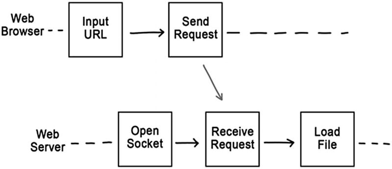
Take, for example, a web browser. The user commands the browser to navigate to a given URL. The browser has just executed two steps: input a URL from the user and send a request to the web server. Since these steps happened in the same process, we know that one happened before the other: “input URL” happened before “send request.”
Now let’s look at what happens in the web server. When it receives the request, it will load the requested file from the hard drive. The receipt of the request and the loading of the file are two steps within the same process. We can therefore say that the receipt happened before the load.

Order of steps in two processes
Because we are using “happened before” as a stand-in for causality , what we are really asserting here is that the user input caused the file to be loaded. This fits well with our intuition. We can imagine that the user intended for the web server to load the file, and so this causal chain of events served to realize the user’s intent. We might also assume that the web server probably would not have loaded that particular file, had the user not entered the URL. But intent and might-have-been are difficult to reason about. “Happened before,” however, is very clear.
We can clearly state when we know one step happened before another. We can also clearly state when we have no idea.
Concurrency
While it was possible in our previous example to say for certain that user input happened before loading a file, it will not always be the case. Some steps happening in different processes will not be so easily put in order, even using the transitive property.
No causal connection between “open socket” and “input URL”
This definition of concurrent is a bit different than others that you might have heard. Concurrent operations in a multi-threaded system might be running in parallel. You have the sense that if two events are concurrent, then they happen at the same time.
By Lamport’s definition of concurrent, we don’t know whether two steps indeed happened at the same time. They could have been separated by a large span of actual time on a physical clock. It could be, for example, that the web server opened the socket hours before the user input the URL. In fact, that is quite likely. But what could be and what is likely do not hold sway in this conversation. It is precisely the fact that we cannot know that makes these two events concurrent.
In a very real sense, concurrency is what makes distributed systems so difficult to think about. If there were no concurrent steps, we could put all of the steps in order. If every step can be ordered relative to every other step, then we would end up with a totally ordered sequence. It would be much easier to think about that kind of system, because it always behaves as if the whole network is running on a single machine.
While a totally ordered system would be easier to think about, it would not have the properties that we desire in a distributed system. It would not scale as we added more hardware, since totally ordered steps cannot be run in parallel. It cannot autonomously serve clients in different locations, because the steps the program takes to serve one client would need to be put in order with others in real time. And it would not allow for disconnected operation, since the steps running on the disconnected computer would be out of sequence with the rest of the network. And so, concurrency is both the hero and the villain of this story .
Partial Order
If you were to compare any two steps running in the same process , you could tell which of the two came first. Those steps are totally ordered. They happen in sequence.
If, however, you compare two steps running in different processes, you might be able to tell which came first. If one preceded the sending of a message, the receipt of which preceded the second, then the transitive property tells us that the first happened before the second. But if that is not the case—if the two steps are concurrent—then you cannot tell which came first. Because sometimes you can tell and sometimes you can’t, the execution of steps in a multi-process system is said to be partially ordered.
Since we are using “happened before” as a stand-in for causality, we can say that causality itself is partially ordered. Some things are causally related: we can clearly say which is the cause and which is the effect. The user input of a URL into a browser caused the web server to load a file. But some things are not causally related. The web server opening a socket did not cause the user to input a URL, nor did the input of the URL cause the web server to open a socket.
Partial order imposes fewer constraints on a system than does total order. It frees up some steps to happen in parallel. It permits devices to act autonomously while disconnected. It gives nodes the ability to act independently without constant synchronization. Recognizing that causality is partially ordered gives us a powerful tool for analyzing distributed systems. We can better understand their capabilities as well as their limitations. And we can make better choices about trade-offs between the two.
The CAP Theorem
Probably the most famous mathematical idea in all of distributed systems is the CAP Theorem. It was postulated by Eric Brewer at the 2000 Symposium on the Principles of Distributed Computing.2 Formally proven by Seth Gilbert and Nancy Lynch in 2002,3 the CAP Theorem relates the ideas of consistency, availability, and partition tolerance. It is often quoted as saying you can only have two of the three.
Consistency means different things in different contexts. Unfortunately, as it usually appears, it doesn’t have a very useful definition. For example, if you’re familiar with relational databases, then you probably first heard of consistency as it relates to the ACID properties of a transaction: atomic, consistent, isolated, and durable. Atomic is easily defined as all or nothing. Isolated simply means that concurrent transactions don’t affect one another. And durable means that the change persisted.
But consistent in this context is not so easy to define. The working definition is that a consistent transaction is one that does not violate any invariants. It “commits only legal results.”4 The trouble is that the invariants that define a legal result come from two sources: the database management system and the application. Database management system invariants include guarantees like “primary keys are unique” and “foreign keys reference rows that exist.” Application-defined invariants, when they exist at all, are defined in terms of the problem domain, such as “all balances are zero or positive.” If we were talking only about the well-defined guarantees generally adopted by database management systems, we might have some chance of proving some generally applicable theorems. But with all of the choices that an application can make in determining its own domain-specific invariants, we find it very difficult to write a meaningful proof. Therefore, we will use a more precise definition.
Defining CAP
Consistency
That’s very different from the definition used in ACID. In fact, you could argue that it’s closer to atomic than to consistent. Either both of the nodes have the latest version of a value, or neither does. But where atomic—and indeed each of the ACID guarantees—is about changes to a single database, consistent in CAP is about nodes in a distributed system.
Availability

Partition tolerance
Armed with these definitions, we can finally state the assertion of Brewer’s conjecture. No distributed system, no matter what algorithm it uses, can simultaneously guarantee consistency, availability, and partition tolerance at any given interval. If during that interval the network is partitioned, then the system will either be inconsistent or unavailable.
This is one of those delightful theorems that challenge you to find an algorithm that works, like Gödel asking you to write a formula that determines whether another expression is true, or Turing imploring you to write a program that determines whether another program terminates, or two generals commanding you to find a reliable way for them to communicate. The proof doesn’t have to guess what you might come up with. It can simply demonstrate, by pain of logic, that whatever you’ve dreamed up will not be equal to the task .
Proving the CAP Theorem
Imagine that you have a system made up of different computers, which we’ll call nodes. Each node has its own internal state. That state, however, is invisible to us. The only thing we can do as an outside observer is to send messages to the nodes and see how they respond.
The message that we will send to the nodes will be read and update. If we send a node a read, it will send us back a value. If we send it an update, it will presumably write down the value and then respond with confirmation. I say presumably, because we can’t really see its internal state.

Update and read
Be careful here. We can’t really tell what these nodes are doing. Their internal operation is left unconstrained. That is important for the proof to be general. If we dictated that they truly were storing internal state, that would limit the kinds of algorithms we could make assertions about.
Similarly, the messages read and update do not constrain our choice in the algorithm either. We do not have to devise a way to send reads and updates to achieve consistency. In fact, these two messages might not even be used by the algorithm. They only exist as a way of setting up a test.
Test an Algorithm
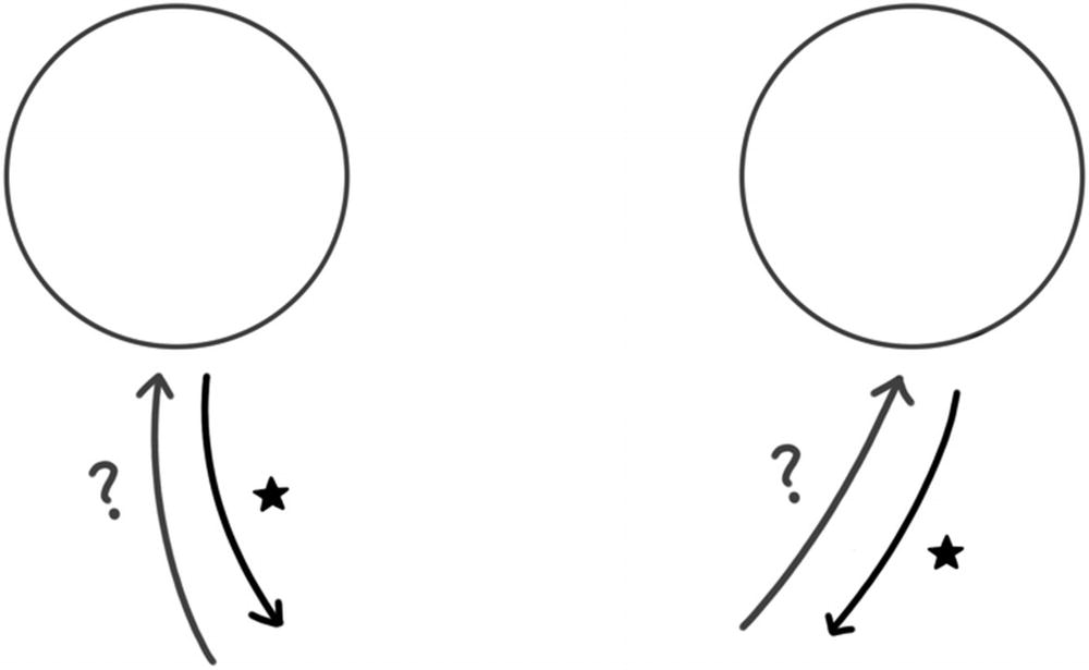
And so, this is the challenge. I ask you to provide an algorithm. You can devise any algorithm you like. You choose the steps. You choose the data structures. I will load this algorithm into two nodes. They communicate with one another by passing messages between them. You choose what messages they will use.
Then, I’ll run a test. I will begin by observing that the nodes are initially consistent. I can tell that they are consistent by sending read messages to each and observing that they return the same answer.
Next, I’ll send one of them an update and wait for it to respond with confirmation. Since it confirmed, I can test the contract by sending that same node a read. If it is behaving properly, it will return that value I just sent it. In about half of the tests, I’ll perform this check. I’ll reject your algorithm if it ever fails to uphold the contract.

Test the algorithm
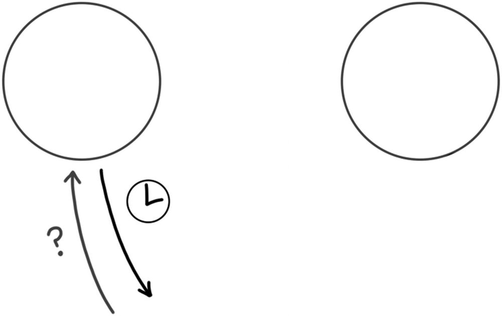
But that’s where I play my trick. During the test, I will create a network partition. The two nodes will not be able to communicate with one another during this interval. The partition will last just a little bit longer than the duration you defined. While communication will eventually be restored, it will not be fast enough for the algorithm to exhibit availability and still be consistent.
- 1.
The first node might block during update until it can communicate the value and then confirm the result. If so, then update takes longer than the specified interval, and so the system is not available.
- 2.
The second node might block during read until it can retrieve the value from the first. If so, then read takes longer than the specified interval, and so again the system is not available.
- 3.
The system might decide to return before the interval has expired. If so, there was no way that the value I updated will be able to propagate to the second node to be read. The second node cannot return the same value as the first, and so the system is not consistent.

Three possible behaviors when the network is partitioned
During this interval of network Partition, the system cannot be both consistent and available. And so, it seems that we are doomed to choose.
Eventual Consistency
If we cannot expect different nodes within a distributed system to have the same state, then what can we hope to achieve? How can we get any work done if we get a different answer from every node that we ask?
Consistency at any given instant may be out of our reach, but all hope is not lost. We can achieve consistency if we wait long enough. Eventually, nodes will come into agreement with one another. This is a concept referred to as eventual consistency.5
While it might be desirable to demand consistency at any given instant, it might not be practical. If we loosen our constraints, we find that we can achieve a much more palatable trade-off. Instead of insisting upon consistency at every given instant, perhaps we can tolerate a lesser degree of agreement. The conversation needs to get a bit more nuanced.
Kinds of Consistency
Marc Shapiro, a researcher at the French National Institute for Computer Science and Control Science (Inria), and Nuno Preguiça, associate professor at Faculdade de Ciências e Tecnologia da Universidade (FCT), sought to understand consistency trade-offs at a formal level. They had each designed special-purpose solutions to achieve eventual consistency, including Treedoc, a replicated data structure for collaborative text editing.6 Each one of these projects required its own formal proof. They wanted a more general result.
Based on their prior results, Shapiro and Preguiça, together with their colleagues, identified three different kinds of consistency.7 The distinctions among them lead to the general result that they sought. They redefined the kind of consistency used in the CAP Theorem as strong consistency . That is the guarantee that all nodes will report being in the same state at any given time. They used the term eventual consistency, on the other hand, to mean that nodes will eventually reach the same state, as long as they can continue to talk to one another. This may require some additional consensus algorithm, such as conflict resolution.
The reliance upon consensus algorithms introduces more than a small degree of overhead. The nodes might need to elect a master to make the final decision, introducing a bottleneck. Or they might run a complicated and chatty algorithm like Paxos to determine by majority decision what the final state shall be. For these reasons, Shapiro and Preguiça decided to distinguish a third kind of consistency. Strong eventual consistency promises that all nodes reach the same state the moment they all receive the same updates. The nodes do not need to talk among themselves to reach a consensus and resolve conflicts.
The CAP Theorem showed us that strong consistency is incompatible with availability. Allowing for consensus algorithm means that the eventual consistency may incur some undesirable overhead. And so, we, like Shapiro and Preguiça, will focus our attention on strong eventual consistency (SEC).
Strong Eventual Consistency in a Relay-Based System
With SEC as our stated goal , let’s construct a useful example. Let’s build a distributed system based on relaying messages and see what properties it must have to satisfy SEC.
This distributed system is made up of nodes connected in some kind of network. The network is connected, which is to say that, unless the network is partitioned (which will occur from time to time), there is a path from any node to any other node. These paths don’t have to be direct; they may go through any number of intermediate nodes.
Some nodes receive new information from outside of the network. When they do, they formulate a message that they themselves process and then send along the network to neighboring nodes. When a neighbor receives the message, it processes it and relays to its neighbors. Each node is running some kind of algorithm to determine when to forward a message and to whom. That algorithm guarantees that eventually, every node will receive every message.
It’s important to observe that we are explicitly not requiring that every node receive each message exactly once. Nor are we requiring that every node receive the messages in the same order. Whatever forwarding algorithm we come up with only has to ensure eventual delivery.
Now let’s consider the internal state of a node within the distributed system. As the node processes a message, it transitions from one state to another. The message can be viewed as a function, taking the starting state as an input and producing the resulting state as the output. The system is strongly eventually consistent (SEC) if, after seeing all of the messages, all nodes arrive at the same state. We can determine what properties those functions must have in order to achieve SEC.
First, every node’s response to each message must be idempotent. If a node sees the same message twice in a row, then it must end up in the same state as if it had seen it only once. And second, every node’s response to each pair of messages must be commutative. If the node sees two messages in one order, it must end up in the same state as if it had seen them in the opposite order.
Taken together, idempotence and commutativity are sufficient to prove SEC. So long, that is, as every node eventually sees every message at least once. This result is only valid for the kind of relay-based distributed system that we defined. It assumes that messages are forwarded exactly as they are, not filtered, altered, or summarized. We will find a more general result in the next section, but for now, let’s examine this relay-based system .
Idempotence and Commutativity
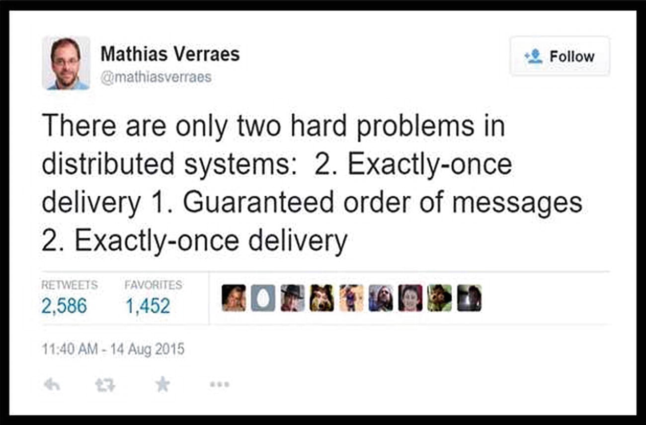
Like all good jokes, this one is absolutely true. It is hard to guarantee that a message is delivered exactly once—not lost and not duplicated. It is even harder to guarantee that messages will arrive in the order in which they were sent.
Network protocols have been invented to specifically try to address these two hard problems. AMQP, for example, is a messaging protocol that can be configured to deliver a range of guarantees. It can be used as a best-effort transport, in which the message is guaranteed to be received no more than once. It can also be tuned up to reliable delivery, which guarantees that a message will be received at least once, but possibly more than once and possibly out of order. With a bit more overhead, it can perform anti-duplication, which attempts to guarantee exactly once delivery. And with a herculean amount of effort, it can serialize messages in a channel, guaranteeing that they will be delivered in the same order they are sent, though you wouldn’t be happy with the performance.
Authors of infrastructure components that rely upon AMQP, such as RabbitMQ, often advise that a consumer be written to tolerate duplicate messages.8 The cost of running a message queue with anti-duplication or serialized channels can be prohibitive. Instead, they recommend that you make your downstream nodes tolerate messages that arrive multiple times, or out of order. That’s precisely what idempotence and commutativity mean.

Idempotent put
A downstream node that tolerates out-of-order messages is said to be commutative. This comes from the mathematical commutative property, which says that an operator has the same result no matter which way its operands are given. The commutative property of addition says that a+b = b+a. Multiplication is also commutative, but subtraction and division are not. In a similar sense, a node is commutative with respect to two messages if it ends up in the same state no matter which message it sees first.
Deriving Strong Eventual Consistency

Non-commutative PUT
Strong eventual consistency requires both idempotence and commutativity. Let’s go back to our working definition of strong eventual consistency to see why this is the case.
A relay-based distributed system is SEC if all nodes, upon seeing the same set of messages at least once in any order, reach the same state. Of course, they must all start in the same state. If the set of messages was empty, the problem would not be interesting: all nodes would still be in the start state. And if the set contained only one message, eventual consistency would only rely upon idempotence. Nodes that receive duplicate copies of that one message will remain in the same state.
And so, we only need to carefully consider the case in which the set contains more than one message. Let’s consider how this might play out. If every node received each message exactly once, then we could argue based on commutativity alone that they would all reach the same state. Or, if every node received each message in order, but some were doubled or tripled, then we could argue based only on idempotence. It’s the fact that things can get jumbled up that causes us to have to stop and consider the possibilities.

Intervening PUT
m1+m2+m3+m1 =
m1+m2+m3
m1+m2+m3+m1 =
m1+m2+m1+m3
We just swapped the m1 and m3 at the end. This moves the duplication of the message one step earlier in the sequence.
m1+m2+m1 =
m1+m1+m2
m1+m1 =
m1
m1+m2+m3+m1 =
m1+m2+m3
And this generalizes to any number of messages. This reduces the problem back down to receiving some set of messages in any order, but with no duplicates. We only need to rely upon commutativity to ensure that any such sequence will yield the same result.
And that is why our PUT example does not exhibit strong eventual consistency. While it is idempotent, it is not commutative. Both properties are required to achieve SEC in a relay-based distributed system.
The Contact Management System
A friend and I created a contact management system , back in the days when personal digital assistants (PDAs) connected to your workstation via RS-232 serial port. At the time, the state of the art was Microsoft’s ActiveSync. We thought we could build a better product.
The solution we came up with was a message store-and-forward system where the nodes (workstations and PDAs) processed messages in an idempotent and commutative fashion. The messages included things like “add contact,” “update contact,” and “delete contact.” Contacts were uniquely identified by GUID, which made add operations trivially idempotent and mutually commutative.

Tombstones
Update operations were the hardest to get right. As with HTTP PUT, the trivial implementation of update is idempotent but not commutative. To solve this problem, we assigned each update message a GUID as well. Each node kept track of the GUID of the most recent update that set a contact’s properties. It would also keep a list of update GUIDs that it saw in the past. When the user changed a contact, it would add the current GUID to the list of past GUIDs and then generate a new current GUID. It included both the current GUID and the list of past GUIDs with the update message.
When a node received an update, it would first check whether that update’s current GUID was already in its own list of past updates. If so, it would ignore the update. If not, it would perform the opposite check: was its current GUID in the message’s list of past GUIDs? If this second check passed, it would accept the update, taking the entire list of past updates.
As long as one of these two checks pass, then updates commute with one another. When received out of order, the future update will deliver the GUID of the past update. The past update would subsequently be ignored.

Compare past and current GUIDs
In addition to merging the properties, the node would also merge the GUIDs. The list of past GUIDs was the union of the current and incoming lists. And the current GUID? That’s where our data structure was a little more complicated than what I first described. The current GUID was also a list. Usually it contained only one element. But after a merge, it contained two (or even more if additional concurrent updates were detected).
This merge is commutative (ignoring concatenation order, which we were happy to do). Each side of the concurrent update would perform the merge upon seeing the other’s message. They would both get the same list of past GUIDs, and they would both get the same list of current GUIDs. When the user subsequently edited this merged contact, both of the current GUIDs would be added to the past list. And so both sides would happily replace its automated merge with the user’s manual one .
Replaying History
This solution worked pretty well. It was strongly eventually consistent (though we didn’t know that term at the time). We proudly showed prospective buyers that we could disconnect a PDA, make changes, and then sync it back up. After all of the messages flowed back and forth, all clients had the same list of contacts in the same state.
During the synchronization process, however, things looked a little sketchy. If a large number of changes had happened on one side, all of those edits would replay before our eyes on the other. Given the speed of networks at the time, you could easily read the list of names as they were added, modified, and subsequently deleted while history replayed on the device.

A new device is introduced to the transaction pipeline
My friend and I never sold an installation of this contact management system. In the end, it proved to be just as clunky as the Microsoft product that we were competing against. Perhaps we could have found a way to prune history, or to download snapshots. But if we had known about conflict-free replicated data types, they would have offered a better solution.
Conflict-Free Replicated Data Types (CRDTs)
Idempotence (ignore duplicates)
Commutativity (don’t depend upon order)
Prove these properties about the way nodes process messages, and you already have a very reliable system. I have built many systems using exactly this technique. It pairs well with infrastructure components such as Amazon SQS, Rabbit MQ, and MSMQ that ensure broadcast and delivery of messages. It requires only a minimum set of guarantees from those components, helping them to work at scale without becoming over-constrained.
But this isn’t the most general result. We can optimize our distributed system further if we allow nodes to modify messages. Instead of requiring that a node forwards exactly the same messages it received, we can allow the node to summarize its knowledge and send fewer messages. This is the strategy employed by conflict-free replicated data types (CRDTs).
State-Based CRDTs
Shapiro, Preguiça, and colleagues described two general solutions to the strong eventual consistency problem: state-based CRDTs and operation-based CRDTs. Operation-based CRDTs require a delivery protocol that ensures once-and-only-once delivery and preserves causal order. We would prefer to find a solution that does not place so high a constraint on infrastructure components. Fortunately, state-based CRDTs have no such restriction. State-based and operation-based CRDTs can each emulate one another and are therefore equivalent. For these reasons, we can put aside operation-based CRDTs for this discussion and focus entirely on the state-based variety.
A conflict-free replicated data type is a data structure that exists not at one location, like a typical abstract data type; it exists in multiple locations. Each node in a distributed system has its own replica of the CRDT. Operating on a replica of a CRDT closely meets our requirements for location independence. Each replica can serve queries in isolation, without communicating with other replicas. And each replica can process commands that immediately alter its state. The effects of these commands will be shared with other replicas in an eventually consistent manner. All replicas will converge to the same state when all updates have been delivered.
The key is to understand what it means for an update to be delivered.
Partially Ordered State
It must support a “happened before” (causality) relationship that defines a partial order.
All updates must increase the state in that partial order (the previous version “happened before”).
It must support a merge operation that takes two states and produces a new one that is greater than both of them (both previous versions “happened before” the merged version).
To be useful, the “happened before” relationship should help us detect concurrent updates. We want to avoid creating a total order and instead capture the partial order inherent in causality.
Unlike our relay-based distributed system, updates do not have to be idempotent or commutative. That’s because updates will be executed only on a single replica. Within a single process, we can easily control how many times and in what order updates are applied. A CRDT does not rely upon message relay like the system we just analyzed.
Shapiro, Preguiça, and colleagues proved that these three conditions are sufficient to guarantee SEC. All replicas will converge to the same state after all updates are delivered. So, what does it mean for an update to be delivered to a replica?
Causal History
When we examine the state of a replica within a single process , we will find only two operations that cause it to change: updates and merges. An update occurs when that node executes some command from outside the network. Perhaps the node is running a client application and responding to user input. A merge occurs when another node shares the state of its replica. This happens on the receive operation of a network communication.
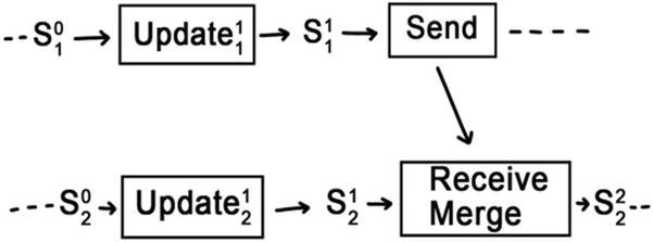
Both updates are in the causal history of s22
- 1.
All updates that have occurred previously in that node
- 2.
All updates in the causal histories of the states that were merged from other nodes.
Remember, the updates themselves are not shared between nodes. Only the resulting states. The necessary conditions imposed by partially ordering the states ensures that they have just enough information about the updates that were performed on them.
And so now we can finally answer the question. What does it mean for an update to be delivered to a replica? It means that that update is in the causal history of its current state.
Vector Clocks
That’s a lot to process . Let’s make it a bit more concrete. How could we have implemented the contact management system as a CRDT? For simplicity, we will look only at the update contact case, which changed the properties of a contact. We’ll represent each contact as a CRDT, where each workstation, PDA, and server node have its own replica.
Let’s start by defining the state. Each contact is going to have a set of properties, like name, phone number, and email address. We will store those in the state.
By our first condition, the state needs to support a “happened before” operator to give us causality. Clearly just looking at the properties of a contact, we cannot tell which of two versions came first. For that, we will need to keep some sort of version number. A simple monotonically increasing version number would satisfy our first and second conditions. We will be able to see which version came first, and we will increase the version number with each update.

A vector clock as part of the contact CRDT
To compare two vector clocks, we compare each node’s version number. If all of the version numbers in the first vector clock are less than or equal to the second, then the first one “happened before” the second. This is a partial order, because it’s possible for one node’s version to be lower in one, while another node’s version is lower in the other. When this happens, the two clocks are not causally related.

Node 2 updates the email of a contact and bumps its own version number
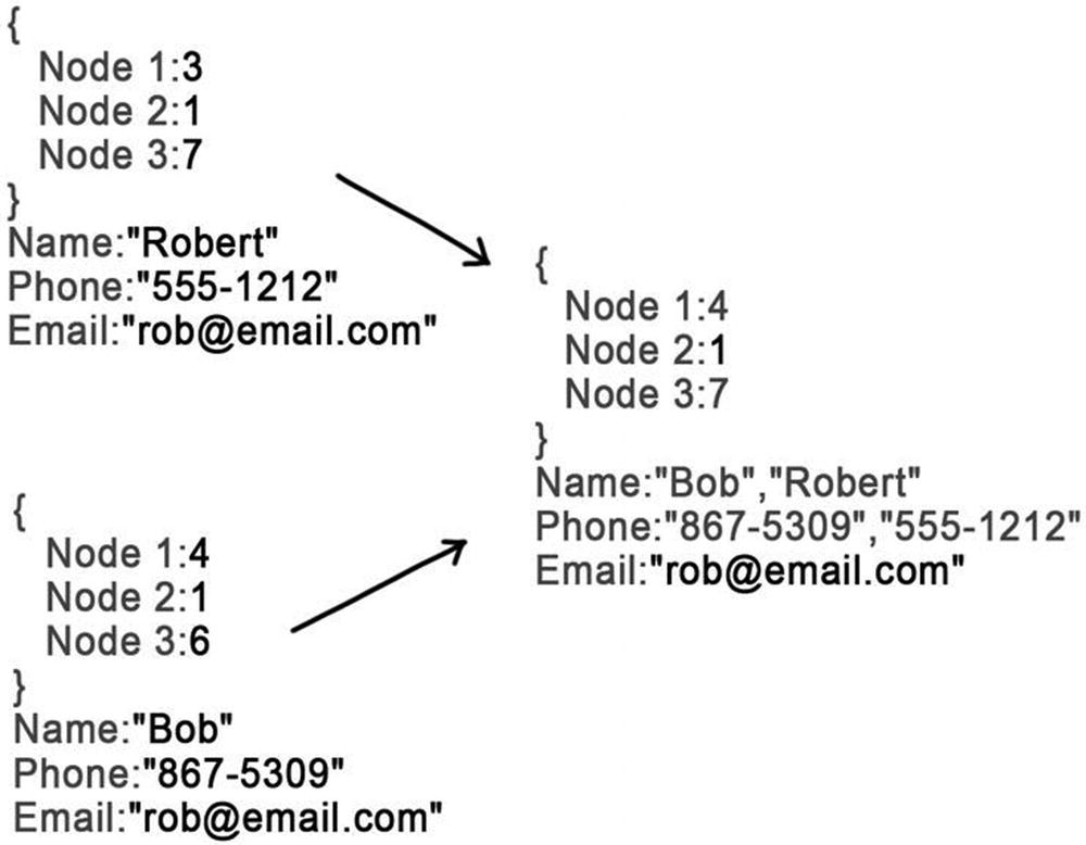
Merging two contacts takes the maxima of all version numbers
We can see that vector clocks satisfy the necessary conditions for SEC. Since we put a vector clock into the state of our CRDT, we have a way to compare two versions to see which one happened before. Incrementing one version number when we update produces a vector clock that is greater than the previous one, so updates increase the state. Merging two vector clocks produces a set of numbers that are all greater than or equal to the previous two vector clocks, and so merge produces a state greater than the source states.
Most importantly, vector clocks capture the causal history of the replica. During a merge, we can detect concurrent updates. If all version numbers in the vector clock of one of the two states are greater than or equal to the other one, then that state represents the more recent version. The values of the contact’s properties will simply be copied from the greater of the two. But if neither vector clock “happened before” the other, then a concurrent update has occurred. That tells us that we need to merge the contact’s properties.
A vector clock is a tool for building state-based CRDTs. It gives us a way to define a partial order between states that supports update and merge operations. When used properly, replicas that include a vector clock will converge to the same value, once all updates appear in their causal history.
If my friend and I had built the contact management systems using vector clocks, then introducing a new device to the system would be a simple download. It would get only the current state of each contact and the vector clock representing the causal history of that state. When a user makes a change on this new device, it would simply add itself to the vector clock at version 1 and share its new value.
A History of Facts
Vector clocks are not the only conflict-free replicated data type. Any data structure that is partially ordered, increases on update, and computes the least upper bound on merge can be used as a CRDT. Researchers have already defined many such data structures for use in different situations.10 With a little work, you can design the CRDT that is exactly right for you.
There is one data structure that is applicable in a surprisingly large number of circumstances. It has a well-defined partial order. It increases on updates. And it comes equipped with a valid merge operation.
I’m talking, of course, about the humble set.
Sets
- 1.
It contains no duplicates.
- 2.
It is unordered.
The first property means that an element is either in the set or it is not. The set does not remember how many times we tried to add an element. The second property tells us that no element comes before or after any other element. The set doesn’t remember the order in which we added the elements.
It’s interesting to observe that set insertion satisfies the two conditions necessary for SEC in a relay-based system. Because of the first property, set insertion is idempotent. If we try to insert an element that is already in the set, it remains unchanged. And because of the second property, set insertion is commutative. Inserting elements in the opposite order yields the same set. These two properties mean that set insertion behaves well in the face of duplicated or out-of-order messages.
Idempotence and commutativity are not required for using a set as an operation-based CRDT. The properties that are required for CRDTs are partial order, increasing updates, and a merge that computes the least upper bound. As long as we do not allow elements to be removed from a set, we can easily achieve all three.
Partial Order
Sets are partially ordered under the subset relationship. One set is a subset of another if it only contains elements that can be found in the other one. If we use subset as “happened before,” then we have defined a partial order.
Take, for example, the set {![]() ,
, ![]() ,
, ![]() }. It is a subset of {
}. It is a subset of {![]() ,
, ![]() ,
, ![]() ,
, ![]() }. Every element in the first is also in the second.
}. Every element in the first is also in the second.
Now consider a third set {![]() ,
, ![]() ,
, ![]() }. It is also a subset of the second. But neither the first nor the third is a subset of the other. The first set contains an element not found in the third (
}. It is also a subset of the second. But neither the first nor the third is a subset of the other. The first set contains an element not found in the third (![]() ), and the third contains an element not found in the first (
), and the third contains an element not found in the first (![]() ). Therefore, they are not related under the subset relationship.
). Therefore, they are not related under the subset relationship.
The fact that some sets can be compared while others cannot is what makes this a partial order. We can use that partial order to represent causality. A subset “happened before” a superset .
Update
The only update operation that we will allow on a set is an insert. If you try to insert an element that the set already contains, then the set is unchanged. But if the element was not already in the set, then the new set has everything that was in the old set plus one additional item. So set insertion, when it modifies the set, increases its value within the partial order.
If you think about the set as containing all of the knowledge of a replica, you can see how set insertion increases that knowledge. The replica still knows everything that it knew before. But after the update, it now knows a little bit more.
This also illustrates how a set can represent the causal history of a replica. Recall that the causal history of a replica includes all of the updates that have occurred in its past. By enumerating the elements of a set, you can clearly see all of the insertions that have occurred over time.
Merge
A valid merge operation in a CRDT will compute the least upper bound of the two values. The least upper bound of two sets under the subset partial order will be the set that contains every element from both sides. It will be a superset of each one. To compute the least upper bound, we simply have to take the set union.
Consider again the two sets {![]() ,
, ![]() ,
, ![]() } and {
} and {![]() ,
, ![]() ,
, ![]() }. Neither is a subset of the other. But we can compute the smallest set that is a superset of both of them. That will be the set union: {
}. Neither is a subset of the other. But we can compute the smallest set that is a superset of both of them. That will be the set union: {![]() ,
, ![]() ,
, ![]() ,
, ![]() }.
}.
This follows our intuition about a merge, as well as the conditions required for SEC. If one node merges all of a remote node’s knowledge into its own, then it ends up with the union of the two. Knowledge grows as a result of that merge.
Thinking of this as the combination of two causal histories also makes intuitive sense. The causal history after a merge includes all of the updates that occurred both locally and remotely.
Historical Records
Let’s formalize this intuition about a set representing the causal history of a replica. Instead of looking at sets of transportation emoji, let the elements in the set be actual historical records.
When a user performs an action at a node, we capture that action as a historical record. We make note of what they were trying to do, what they were trying to do it to, and what options or parameters they chose while doing it. The record is simply a structure that collects all of this information. It captures all of the pertinent data that was part of the user’s decision.
- 1.
We need to distinguish between similar records.
- 2.
We cannot remove a record once it is inserted into the set.
- 3.
We cannot change a record that is already part of the set.
- 4.
Some of the records are related to one another.
These four observations give rise to the rules of historical models.
Distinguishing Between Records
Revisiting the contact management system, we can identify the first action that a user might perform at a node. They will want to create a new contact. When a new contact is created, it doesn’t have any properties. Those can be changed later.
{ ContactCreation }
When they try to create a second contact, however, they run into a problem. The record ContactCreation already exists in the set. It cannot be inserted again.
{ ContactCreation(1), ContactCreation(2) }
The problem with this strategy becomes apparent when we merge one node’s causal history with that of another. Merge is accomplished with a set union. If they were both generating identifiers using an auto-incrementing counter, then they would produce the same identifier for different contacts. The set union would merge different contacts into one.
{ ContactCreation(74aac247-a86a-4af8-9db4-cf1387f8a1fb),
ContactCreation(5853e3fe-059a-4180-af0a-f969260be882) }
And so we have discovered that a historical record is uniquely identified only by its content. It has no other identifier. This is to ensure that causal histories merge in a location-independent manner.
Removing a Record
{ ContactCreation(74aac247-a86a-4af8-9db4-cf1387f8a1fb) }
But this strategy won’t work. It violates the second condition of a state-based CRDT. Update operations may only increase the state of a replica within the partial order. Removing an element from a set creates a subset, not a superset. This takes the state backward in causal time.
It becomes apparent that we’ve made a mistake when we share state with other nodes. Suppose the user creates a contact, and then their device shares its state with another node. That contact creation is now part of the other node’s replica.
Now suppose that the user removes that contact, and the node incorrectly represents that by removing it from the set. When the remote node at some point in the future shares its state with the user’s node, the replica sets will be merged. The contact that they had deleted will suddenly reappear. Just search for “deleted contact reappears” in your favorite search engine to see just how common this bug is.
{ ContactCreation(74aac247-a86a-4af8-9db4-cf1387f8a1fb),
ContactCreation(5853e3fe-059a-4180-af0a-f969260be882),
ContactDeletion(5853e3fe-059a-4180-af0a-f969260be882) }
We have restored the condition that updates increase state within the partial order. This new set is a superset of the prior one. And merging state with other nodes will never cause the contact to reappear.
We have just discovered that a historical record cannot be deleted. A record can represent the deletion of an entity. But it cannot be removed from causal history.
Changing a Record
{ ContactCreation(74aa…),
ContactModification(74aa…, “Bob”, “555-1212”) }
{ ContactCreation(74aa…),
ContactModification(74aa…, “Robert”, “555-1212”) }
We can already see why that doesn’t work. The new set is not a superset of the original one. This violates the second condition: updates must increase state in the partial order. We have, in fact, created a new set that is not causally related to the old one.
{ ContactCreation(74aa…),
ContactModification(74aa…, [node1: 1], “Bob”, “555-1212”),
ContactModification(74aa…, [node1: 2], “Robert”, “555-1212”) }
We have discovered that once a record is part of history, it cannot be modified. We can add a new record that represents a modification to an entity, but the old records must remain.
Since we already have a complete set of the historical records, the vector clock is a bit redundant. Remember, vector clocks help us to turn a simple data structure into a CRDT. It captures the partial order of causality. But now that we are working with a set of simple data structures, we can rely upon the set to capture causality. We have the opportunity to optimize a bit.
Records Are Causally Related
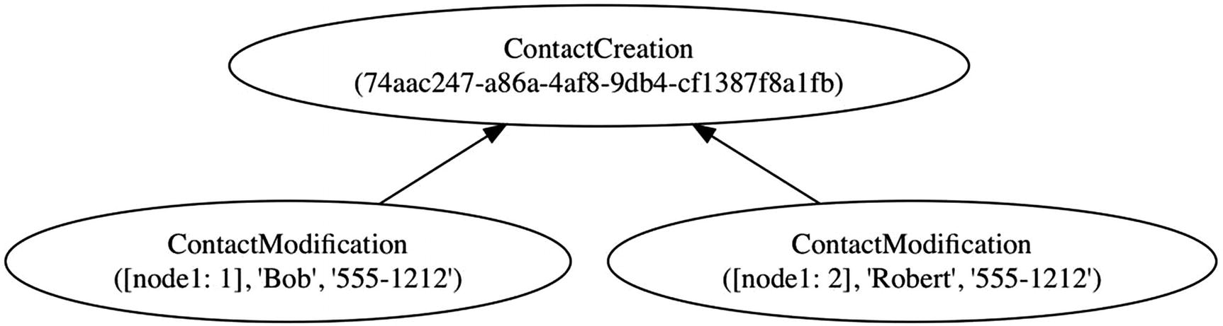
Contact creation precedes contact modification
This graph is still a set. Every vertex of the graph is a historical record in the set. All we have done is replaced the implied relationships of common GUIDs with explicit arrows.

Vector clocks are replaced with explicit arrows
Changing the vector clocks to arrows preserves the partial order between modifications. It is still easy for us to compare two ContactModification records to see which one came before the other. If we can trace a path from one to the other along the arrows in the correct direction, then the record at the head of the last arrow “happened before” the record at the tail of the first one.
The graph captures the partial order of causality.
This is true in general, not just for the modifications. ContactCreation happened before ContactModification . The user must have created a contact before setting its properties. If the contact wasn’t created on the local node, then it must have been created remotely and merged into the set. By Lamport’s causality, even that remote creation happened before the local modification.
Benefits of Explicit Causality
We have captured the causal relationships between historical records as arrows in a directed graph. Doing so is more than just an optimization. It also enforces preconditions of the user’s actions. A user cannot modify the properties of a contact that hasn’t been created. Nor can they delete one that doesn’t exist. When the causal relationships between records were only implied by a shared GUID, the data structure did nothing to help us ensure that these preconditions were met. But now that it explicitly captures the arrows, these preconditions are enforced by the existence of the record at the head.
Another benefit is that we have just traded away less important information for more important information. The vector clock included the names of the nodes at which modifications were made. It needed this information only so that a node knew which version number to increment on update. After that, the names of the nodes are unimportant. The arrows discard the names of the nodes in favor of explicit references to prior versions. It doesn’t matter whether that prior version was produced on the same node, or arrived as the result of a merge.
In exchange for discarding unimportant information, the explicit arrows provide us with much more important information. They tell us how an entity has changed over time. This is useful in computing a better merge.

A graph after merging concurrent modifications
The partial order among modifications shows us that the two leaves of the graph are not causally related. Neither one happened before the other. We therefore need to merge the two sets of properties to display to the user.
The concatenation-based merge that we did before would produce a contact with two names and two phone numbers. If all we had were two data structures and two vector clocks, this is the best we could hope to achieve. But having the graph gives us a third data point. We can see the nearest common ancestor of the two leaves.
name: “Robert”
phone: “867-5309”
This three-way merge happens only on display. The set (or graph) of historical records is not modified in any way. Furthermore, all nodes perform this three-way merge in exactly the same way. They all have the same graph, so they will all compute the same result. So even when the history captures causally unrelated records, it does not result in a conflict. Every node converges to the same value.
With this final observation , we have discovered that historical records are related to one another explicitly. This relationship captures the partial order of causality. The record at the head of the arrow happened before the one at the tail.
Historical Facts
Because these records are no longer simple flat data structures, I hesitate to call them records anymore. Nor do I like referring to them as historical events, as that evokes Event Sourcing. Event Sourcing captures a totally ordered sequence of historical events, but does not capture explicitly the relationships between historical events. And so I refer to these elements of the causal set as historical facts.
The arrows point toward the predecessor of a historical fact. The earlier fact preceded the latter one. The latter, I call the successor. Arrows are only inserted into the graph with the successor, never afterward. This enforces preconditions, preserves the partial order of the causal relationship, and has the extra benefit of preventing cycles. The contents of a fact combined with its set of predecessor arrows are all that distinguish it from other facts. Because facts have no extrinsic identity, nodes can refer to facts in a location-independent manner. The entire causal set is what I call the historical model.
A historical model is a state-based CRDT that captures the causality among historical facts as a directed acyclic graph. The arrows of the graph impose a partial order that shows which facts happened before which other facts. Facts in the graph can be referenced, queried, and used with no dependence upon the location of the node.
The graph supports two operations: insert and merge. Inserting a new historical fact moves the graph forward along the causal timeline, because the resulting graph is a superset of the original. Merging two historical models computes their least upper bound and therefore helps remote replicas achieve strong eventual consistency.
Conclusion
We have identified the properties that a distributed system must have in order to be location independent. They must exhibit location independence both in identity and in behavior.
A location-independent identity does not imply any affinity of an object upon its location of origin. Any node should be able to generate and compare a unique immutable identity for a new object without communicating with other nodes. This reduces latency and increases autonomy of isolated nodes within a distributed system.
Location-independent behavior permits a node to query and transact with replicas of objects in isolation. These replicas achieve strong eventual consistency when all replicas converge to the same state once all updates are delivered. This can either be achieved by means of an idempotent and commutative relay system or by a more sophisticated conflict-free replicated data type.
From these constraints, we derived a set of rules that help us to define systems that operate in a location-independent fashion. I call this set of rules Historical Modeling. The reasoning laid out in this chapter demonstrates that a historical model satisfies the requirements for strong eventual consistency.
But before we code up a historical model, we should understand exactly what they tell us about the systems we intend to build. Let’s explore these rules first as a means of analyzing a problem. Among other things, the rules quickly reveal when we make the assumption that data has a location. This analysis will uncover potential problems long before they have a chance to cause issues in production.