
4
Automated TSR Using DNN Approach for Intelligent Vehicles
Banhi Sanyal*, Piyush R. Biswal, R.K. Mohapatra, Ratnakar Dash and Ankush Agarwalla
Department of Computer Science, NIT, Rourkela, India
Abstract
Traffic Sign Recognition (TSR) system has become an indispensable component for intelligent vehicles. The primary focus is to develop an efficient DNN with a reduced number of parameters to make it real-time implementable. The architecture was implemented on GTSRB. Four variations of Neural network architectures: Feed Forward Neural Network (FFNN), Radial Basis Function NN (RBN), Convolutional Neural Network (CNN), and Recurrent Neural Network (RNN) are designed. The various hyper-parameters: Batch Size, Number of epochs, Momentum, Initial Learning Rate of the architectures, are tuned to achieve the best results. Extensive experiments are performed to study and improve the effects on efficiency. The effects of other techniques such as validation split (0.1 and 0.2) and data augmentation are also investigated. All results are tabulated to learn the effects of different techniques. The best performing model was selected as the real-time implementable architecture of our research. Four pre-trained models, namely LeNet, GoogleNet, ResNet, and AlexNet were also implemented on the same database for comparative studies. Various other schemes of other researchers have also been provided. The comparative studies prove the supremacy of our proposed architecture.
Keywords: Traffic sign recognition, DNN, validation split, pre-trained models, neural network
4.1 Introduction
Accidents are a major reason of death and collateral health damage per year around the globe. Though human visual systems have developed systems for recognition purposes (with a few limitations), still, drivers are vulnerable to various human factors of contributing to roads accidents which are:
- Over-speeding.
- Rash driving.
- Violation of rules.
- Failure to understand signs.
- Fatigue.
- Alcohol.
Thus there is an increased interest and dependence on Autonomous driving automatic systems (ADAS) and Intelligent transport systems (ITS) during the recent years. These intelligent vehicles have automated systems which reduce human interference and dependence. A few such techniques are anti-theft cars, automatic parking of cars in parking lots or other areas, maintaining safe distance at all times from surrounding vehicles and traffic sign recognition (TSR).
In this chapter, we will be focusing on TSR in ADAS systems. The classical problem of TSR has the objective to recognize traffic sign from a given still image or from a video frame. Traffic signs are provided at the side of the roads to inform drivers and pedestrians about state of the road and traffic warnings or guidelines. Different techniques are developed and adopted to aid artificial object recognition systems. The efficiency of human visual systems has given rise to Convolutional Neural Network (CNN) which has been developed mimicking the behavior of the mammalian visual cortex. Studies on the competitive results of various recognition techniques such as CNN, SVM and RF [1]. Lately CNN has given highest efficiency in the ImageNet Challenge [2] and the 2011 IJCNN competition [3, 4]. It is worth mentioning here that TSR suffers various types of challenges. In order to be real-time implementable, architectures should perform reasonably well under such constraints. A few of the challenges include lowered quality of images, occlusion, blur caused due to the speed of the vehicle (motion blur), poor weather conditions and/or lighting conditions. CNN is also known to perform well in various such challenges as well.
The main focus of this chapter is to utilize the efficiency of CNN. An architecture to automatically learn high-level features from images, without the need of hand-crafted features. Four such Neural Network architectures, namely FFNN, RBN, CNN, and RNN are designed. The various hyper-parameters: Batch Size, Number of epochs, Momentum, Initial Learning Rate of the architectures, are tuned to achieve the best results. An extensive set of experiments was conducted to study and improve the effects on efficiency. The effects of other techniques such as validation split (0.1 and 0.2) and data augmentation are also investigated. All results are tabulated to learn the effects of different techniques. The pooling strategies are also varied to obtain the best performing architecture. The best performing model was selected as the real-time implementable architecture of our research. We also implemented four pre-trained models, namely LeNet, GoogleNet, ResNet, and AlexNet, on the same database for comparative studies. Various other schemes of other researchers have also been provided. The comparative studies prove the supremacy of our proposed architecture.
The rest of the chapter is organized as follows. Section 4.2 discusses various state-of-the-art approaches in TSR. Section 4.3 discusses about CNN architecture. All methodology is given in Section 4.4. The experimental results are compared and discussed in Section 4.5. The scheme is analyzed in Section 4.6. The work is concluded in Section 4.7.
4.2 Literature Survey
Many researchers have come forward in the field of TSR. Their contributions address a wide range of challenges efficiently. The various aspects of intelligent vehicles like ADAS [5–7], ITS [8], SLS detection (Speed Limit Sign) [9], Global Navigation Satellite System (GNSS) [10]. Kashihara [11] worked on using Frontal electroencephalogram (EEG) of drivers, to include attention level of driver as a human response to the situation in the automated system. Roters et al. [12] worked on visually impaired pedestrians to cross roads. This research led to include both environmental and human input for an automated system in TSR. TSR recognition has been divided into two approaches widely by different authors: traffic panel detection [13, 14], and panel text recognition [8, 15–18].
In recent years traffic assistance has improved immensely. A comprehensive study has been done on the recent techniques adopted in TSR. The recognition of road signs include two variations. First being recognition of characters [8, 15, 17–19]. The second includes recognition of both characters and digits [18]. The various traditional tools used in detection are for Histogram of oriented gradients (HOG) [20], Support Vector Machines (SVM) for detection in [21]. A few new era techniques are Extreme Learning Machine (ELM) [22], Group Sparse Coding [4] and Hinge Loss Technique [23], Meta-heuristic algorithms and others. TSR signs focused on sign recognition from still images, video [19, 24, 25] or live stream [9, 14, 16, 26, 27].
4.3 Neural Network (NN)
NN is a supervised machine learning technique which has an input layer and an output layer with the presence or absence of in-between hidden layers. The hidden layers are generally a combination among convolutional layers, max-pooling layers, normalization layers, full link layer, soft-max layer and flatten. The weights are initiated randomly and updated in a feedback sequence. Convolutional layers extract local feature patterns. A 3D kernel is used which has a 3D matrix and a bias. The output of this layer is the inner cross product of the corresponding elements of the kernel and the input matrix added to the bias. Let Mx, My be the size of M maps for all the layers and Kx, Ky be the kernel size to be convoluted over the image with skipping factors Sx, Sy and n is the layer number. The output map size is given in Equation 1.
Equation 1:
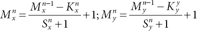
Max-Pooling layers are used for reducing feature vector size and the output is the maximum activation function of non-overlapping kernels of size Kx, Ky. This method is called subsampling and is used to aid the process of classification. ReLU layer applies an activation function such as the max(0, x) function, to product element wise non-linearity. Dropout layer is used to drop random units of weights and biases as the input layer of the next layer to prevent the model to over fit the training data. Full link layers are the layers of CNN where each of the nodes of a layer is connected to each node of the next layer. Soft-max layer is the activation function of the last layer of a CNN and a k-class classification and a multiclass logistic regression. Flatten is to rearrange the output of the previous layer into a one dimensional feature vector. Various preprocessing techniques are applied to the data before applying machine learning techniques. Validation split is splitting the training dataset to fit the model to the training data set while tuning its hyper parameters. Data augmentation is a technique in machine learning with the sole purpose of dataset expansion so as to avoid over-fitting in the neural networks. The competitive results are calculated and compared with current state-of-the-art methods.
4.4 Methodology
The conducted experiments and results are presented.
4.4.1 System Architecture
The proposed architecture was run on a 4GB RAM, Intel Core i3 system.
4.4.2 Database
The German Traffic Sign Benchmarks (GTSRB) dataset has been used in the experiments. GTSRB consists of traffic signs with different resolutions and image distortions and organized into 43 pre-defined classes. Few examples from the video are given in Figure 4.1. A table illustrating the details of GTSRB and other databases in TSR is given in Table 4.1. A wide variety of databases can be observed.
4.5 Experiments and Results
All the conducted experiments and their results are detailed. Four types of neural networks are considered for this work, namely FFNN, RBN, CNN and RNN. To increase the efficiency further, DL approaches like data augmentation, validation split are applied. The validation is split is tested with 0.1 and 0.2. The results of the above experiments are tabulated in Table 4.2. It is noticed that while CNN works well amongst the implemented architecture, RBF fails to make an impression. All the implemented neural networks are discussed in detail in Table 4.3.
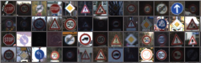
Figure 4.1 Examples from GTSRB.
Table 4.1 Different datasets on traffic signs.
| Databases | Classes | Annotations | Total images | Annotated images | Sign size (in px) | Image size (in px) | Country |
| GTSRB | 43 | 50,000 | 50,000 | All | 15 ∗ 15 to 250 ∗ 250 | 15 ∗ 15 to 250 ∗ 250 | Germany |
| STS | 7 | 3,488 | 20,000 | 400 | 3 ∗5 to 263 ∗ 248 | 1,280 ∗ 960 | Sweden |
| KUL | 100+ | 13,444 | 9,006 | All | 100 ∗ 100 to 1,628 ∗ 1,236 | 1,628 ∗ 1,236 | Belgium |
| RUG | 3 | 0 | 48 | 0 | NA | 360 720 | The Netherlands |
| Strepolis | 10 | 251 | 847 | All | 25 25 to 204 159 | 1,930 1,080 | France |
| IRSDBv1.0 | 49 | NA | 1,691 | All | NA | 3,264 1,836 and 6,000 4,000 | India |
Table 4.2 Efficiency (in %) results for implemented classifiers.
| Classifier | Without DL technique | Data augmentation | Data augmentation with 0.1 split | Data augmentation with 0.2 split |
| FFNN | 81.28 | 83.94 | 84.22 | 86.57 |
| RBN | 50.00 | 56.00 | 57.00 | 57.02 |
| CNN | 81.45 | 85.79 | 86.75 | 87.31 |
| RNN | 58.56 | 68.96 | 70.89 | 78.00 |
Table 4.3 Details of best performing architecture.
| Classifier | Efficiency (in %) | Details |
| FFNN | Training Accuracy: 97.31 Validation Accuracy: 86.38 Test Accuracy: 86.57 | Data augmentation Validation split = 0.2 Epochs = 20 Batch size = 128 Learning rate = 0.01 Momentum = 0.9 |
| RBN | Training accuracy = 57.02 Validation accuracy = 54.89 Test accuracy = 46.99 | Data augmentation Validation split = 0.2 Epochs = 50 Batch size = 128 Learning rate = 0.01 |
| CNN | Training accuracy = 90.01 Validation accuracy = 36.99 Test accuracy = 87.31 Training loss = 28.00 Validation loss = 36.99 | Epoch = 50 Batch size = 128 Learning rate = 0.01 |
| RNN | Training accuracy = 89.00 Validation accuracy = 81.00 Test accuracy = 78.00 | Epochs = 50 Learning rate = 0.05 |
It can be noticed that FFNN epochs are 20 as compared to 50 epochs in other architectures. This is because the increase in epochs in FFNN leads to overfitting. As such test accuracy does not increase with the increase in number of epochs. Therefore, the number of epochs are limited to 20, where it achieves the highest test accuracy. It is evident from the table and that all the architectures perform best at validation split of 0.2. The results and graphs of the architectures (FFNN, CNN, RNN) are all provided. RBN has not been able to give a good accuracy and therefore has not been discussed further. The architectures of each of the NN has been selected through experiments, and only the best performing architecture of each type of NN is provided.
4.5.1 FFNN
The details of the implemented Feed forward neural network (FFNN) are detailed in Tables 4.4, 4.5 and 4.6. Figures 4.2, 4.3 and 4.4 give the graphs (accuracy and loss) and confusion matrix of the same.
Table 4.4 Architecture of FFNN.
| Layer (type) | Output shape | Parameters # |
| Linear-1 | [1,024] | 3,146,752 |
| BatchNorm1d-2 | [1,024] | 2,048 |
| ReLU-3 | [1,024] | 0 |
| Linear-4 | [512] | 524,800 |
| BatchNorm1d-5 | [512] | 1,24 |
| ReLU-6 | [512] | 0 |
| Linear-7 | [256] | 131,328 |
| BatchNorm1d-8 | [256] | 512 |
| ReLU-9 | [256] | 0 |
| Linear-10 | [128] | 32,896 |
| BatchNorm1d-11 | [128] | 256 |
| ReLU-12 | [128] | 0 |
| Dropout-13 | [128] | 0 |
| Linear-14 | [ 43] | 5,547 |
Table 4.5 Detailed parameters of FFNN.
| Type of parameters | Parameters # |
| Total parameters | 3,845,163 |
| Trainable parameters | 3,845,163 |
| Non-trainable parameters | 0 |
Table 4.6 Size details on FFNN.
| Type | Data size |
| Input size (MB) | 0.01 |
| Forward/backward pass size (MB) | 0.05 |
| Parameters size (MB) | 14.67 |
| Estimated Total Size (MB) | 14.73 |
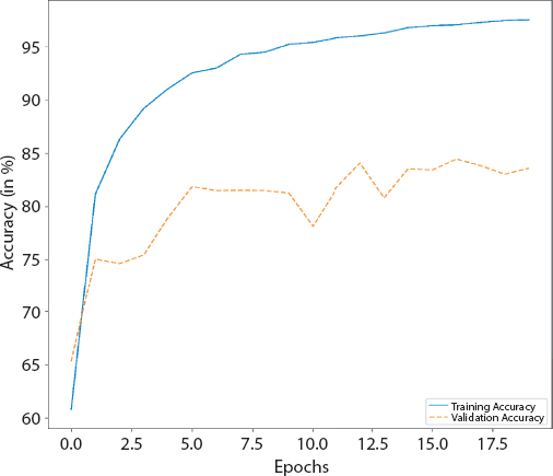
Figure 4.2 Accuracy graph of FFNN.
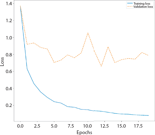
Figure 4.3 Loss graph of FFNN.
4.5.2 RNN
The details of the implemented Recurrent neural network (RNN) are detailed in Tables 4.7, 4.8 and 4.9. Figures 4.5 and 4.6 give curves of RNN. Figure 4.7 gives the confusion matrices of the same. The white bands are the classes where no image was classified into. The whole row in confusion matrix consists of 0s. Hence the normalized value comes out to be very high.
4.5.3 CNN
The details of the implemented Convolution neural network (CNN) are detailed in Tables 4.10, 4.11 and 4.12. Figures 4.8, 4.9 and 4.10 give the graphs (accuracy and loss) and confusion matrices of the same. The white bands in Figure 4.10 are the classes where no image was classified into. The whole row in normalized confusion matrix consists of 0s. Hence the normalized value comes out to be very high.
4.5.4 CNN
CNN gives the most promising results in the previous experiments. As such it is prudent to draw a deeper understanding. The best performing approach of CNN from Table 4.2 is selected and its architecture is varied. A higher performing architecture is attained, the results of which are detailed in Table 4.13. The scheme is discussed in Table 4.14. The details of the improved Convolution neural network (CNN) are detailed in Tables 4.14, 4.15, 4.16, and 4.17. Figures 4.11, 4.12 and 4.13 give the graphs (accuracy and loss) and confusion matrix of the same.
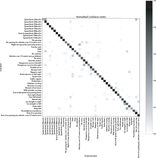
Figure 4.4 Normalized confusion matrix of FFNN.
Table 4.7 Architecture of RNN.
| Layer (type) | Output shape | Parameters # |
| RNN-1 | [[1, 100], [2, 100]] | 0 |
| Linear-2 | [43] | 4,343 |
Table 4.8 Detailed parameters of RNN.
| Type of parameters | Parameters # |
| Total parameters | 4,343 |
| Trainable parameters | 4,343 |
| Non-trainable parameters | 0 |
Table 4.9 Size details on RNN.
| Type | Data size |
| Input size (MB) | 0.00 |
| Forward/backward pass size (MB) | 0.15 |
| Parameters size (MB) | 0.02 |
| Estimated Total Size (MB) | 0.17 |
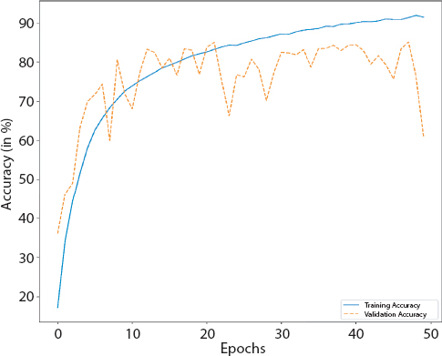
Figure 4.5 Accuracy curve of RNN.
The hyper-parameters were also fine-tuned to achieve better performance. A list of hyper-parameters is mentioned in Table 4.15.
The imapct of change in pooling strategy was also studied and the result is tabulated in Table 4.18. Max-pooling is used currently in the CNN architecture. A fall is noticed in accuracy while changing to average pooling. Hence the pooling strategy is kept as Max-pooling.
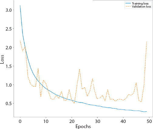
Figure 4.6 Loss graphs of RNN.
4.5.5 Pre-Trained Models
For further experiments we implemented four pre-trained models namely AlexNet, GoogleNet, LeNet and ResNet on GTSRB. The accuracy of each is provided in Table 4.19. We observe that our proposed CNN performs better than all the pre trained models.
4.6 Discussion
Several frameworks and various DL approaches were experimented. A novel DL architecture is proposed to automate multi-class TSR on GTSRB. The comparative results of all various schemes are provided in Table 4.20. The comparative results indicate the supremacy of the scheme against other state-of-the-art works. The architecture was better at automatically learning high level abstractions and thus proved to be superior to others. Further, the proposed model performed better than four pre-trained models namely, AlexNet, GoogleNet, LeNet and ResNet. The results of the pre trained models are tabulated in Table 4.19. Table 4.15 shows the number of trainable parameters in the proposed architecture of 10,649,387 only, as compared to other DNN approaches. In addition to the increased efficiency, the proposed architecture has the following improvements over others: 1) Terminates the need of hand-crafted feature abstractions, 2) Lower number of parameters (10,649,387 only) are employed in contrast to other schemes, 3) Higher accuracy in an optimized recognition time.
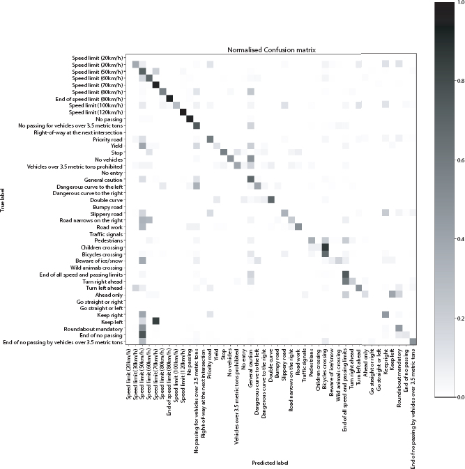
Figure 4.7 Normalized confusion matrix of RNN.
4.7 Conclusion
A DNN is proposed for automated multi-class TSR. The proposed architecture is compared to the results of other architectures. There are pretrained models implemented. A high accuracy of 97.59% was observed. Additionally there are other advantages as well. Lower number of parameters and lower recognition time. The approach overcomes the necessity of hand-crafted features. The architecture can be extended to other traffic sign datasets and other image analysis fields as well.
Table 4.10 Architecture of CNN.
| Layer (type) | Output shape | Parameters # |
| Conv2d-1 | [10, 29, 29] | 1,090 |
| BatchNorm2d-2 | [10, 29, 29] | 20 |
| ReLU-3 | [10, 29, 29] | 0 |
| MaxPool2d-4 | [10, 14, 14] | 0 |
| Conv2d-5 | [20, 10, 10] | 5,020 |
| BatchNorm2d-6 | [20, 10, 10] | 40 |
| ReLU-7 | [20, 10, 10] | 0 |
| MaxPool2d-8 | [20, 5, 5] | 0 |
| Linear-9 | [200] | 100,200 |
| Dropout-10 | [200] | 0 |
| Linear-11 | [90] | 18,090 |
| Linear-12 | [43] | 3,913 |
Table 4.11 Detailed parameters of CNN.
| Type of parameters | Parameters # |
| Total parameters | 128,373 |
| Trainable parameters | 128,373 |
| Non-trainable parameters | 0 |
Table 4.12 Size details on CNN.
| Type | Data size |
| Input size (MB) | 0.01 |
| Forward/backward pass size (MB) | 0.26 |
| Parameters size (MB) | 0.49 |
| Estimated Total Size (MB) | 0.76 |
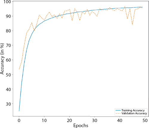
Figure 4.8 Accuracy graph of CNN.
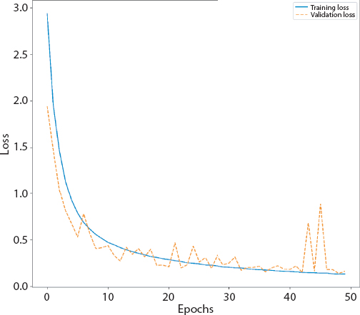
Figure 4.9 Loss graph of CNN.
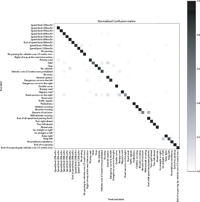
Figure 4.10 Normalized confusion matrix of CNN.
Table 4.13 Accuracy and loss of improved CNN.
| Detail | Accuracy (in %) |
| Training accuracy | 99.92 |
| Validation accuracy | 97.67 |
| Test accuracy | 97.59 |
Table 4.14 Architecture of improved CNN.
| Layer (type) | Output Shape | Parameters # |
| Conv2d-1 | [16, 64, 64] | 448 |
| BatchNorm2d-2 | [16, 64, 64] | 32 |
| ReLU-3 | [16, 64, 64] | 0 |
| MaxPool2d-4 | [16, 32, 32] | 0 |
| Conv2d-5 | [32, 32, 32] | 4,640 |
| BatchNorm2d-6 | [32, 32, 32] | 64 |
| ReLU-7 | [32, 32, 32] | 0 |
| MaxPool2d-8 | [32, 16, 16] | 0 |
| Conv2d-9 | [64, 16, 16] | 18,496 |
| BatchNorm2d-10 | [64, 16, 16] | 128 |
| ReLU-11 | [64, 16, 16] | 0 |
| MaxPool2d-12 | [64, 8, 8] | 0 |
| Dropout-13 | [64, 8, 8] | 0 |
| Linear-14 | [2,048] | 8,390,656 |
| ReLU-15 | [2,048] | 0 |
| Dropout-16 | [2,048] | 0 |
| Linear-17 | [1,024] | 2,098,176 |
| ReLU-18 | [1,024] | 0 |
| Dropout-19 | [1,024] | 0 |
| Linear-20 | [128] | 131,200 |
| ReLU-21 | [128] | 0 |
| Dropout-22 | [128] | 0 |
| Linear-23 | [43] | 5,547 |
Table 4.15 Detailed parameters of improved CNN.
| Type of parameters | Parameters # |
| Total parameters | 10,649,387 |
| Trainable parameters | 10,649,387 |
| Non-trainable Parameters | 0 |
Table 4.16 Size details on improved CNN.
| Type | Data size |
| Input size (MB) | 0.05 |
| Forward/backward pass size(MB) | 2.95 |
| Parameters size (MB) | 40.62 |
| Estimated Total Size (MB) | 43.62 |
Table 4.17 Hyper-parameters of improved CNN.
| Hyper-parameters | Value |
| Batch Size | 50 |
| Number of epochs | 50 |
| Initial Learning Rate | 0.01 |
| Validation split | 0.5 |
Table 4.18 Impact of pooling strategy on accuracy of improved CNN.
| Pooling strategy | Accuracy (in %) |
| Max-pooling (Currently used) | 97.59 |
| Average pooling | 96.99 |
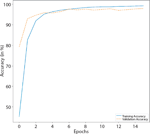
Figure 4.11 Accuracy graph of improved CNN.
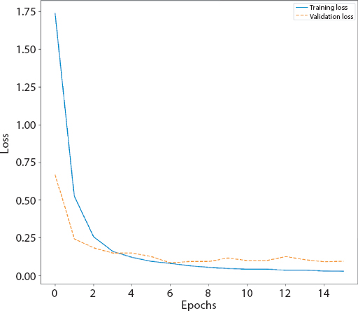
Figure 4.12 Loss graph of improved CNN.
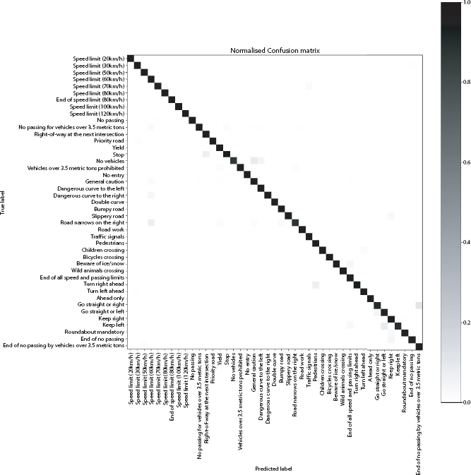
Figure 4.13 Confusion matrix of improved CNN.
Table 4.19 Accuracy of various pre trained models.
| Model | Accuracy (in %) |
| AlexNet | 87.88 |
| Google Net | 72.76 |
| LeNet | 92.12 |
| ResNet | 70.88 |
Table 4.20 Comparative results with state-of-the-art schemes.
| Authors | Scheme | Accuracy (in %) |
| Gudigar et al. [28] | GIST + Graph based LDA + KNN | 96.33 |
| Peng et al. [29] | Autoencoder variant | 90.47 |
| Abdullah et al. [30] | Curvelet + Cuckoo search algorithm | Yellow = 93 Green = 94 Blue = 94 Red = 96 |
| Wicaksono et al. [31] | Gabor wavelet + PCA | 90.55 |
| Sapijaszko et al. [32] | DWT + DCT + MLP | 95.70 |
| Proposed architecture | DNN | 97.59 |
References
1. Stallkamp, J., Schlipsing, M., Salmen, J., Igel, C., Man vs. computer: Benchmarking machine learning algorithms for traffic sign recognition. Neural Netw., 32, 323–332, 2012.
2. Ciregan, D., Meier, U., Schmidhuber, J., Multi-column deep neural networks for image classification, in: IEEE Conference on Computer Vision and Pattern Recognition, pp. 3642–3649, 2012.
3. LeCun, Y., Bottou, L., Bengio, Y., Haffner, P., Gradient-based learning applied to document recognition, in: Proceedings of the IEEE, vol. 86, pp. 2278–2324, 1998.
4. Liu, H., Liu, Y., Sun, F., Traffic sign recognition using group sparse coding. Inf. Sci., 266, 75–89, 2014.
5. Mogelmose, A., Trivedi, M.M., Moeslund, T.B., Vision-based traffic sign detection and analysis for intelligent driver assistance systems: Perspectives and survey. IEEE Trans. Intell. Trans. Sys., 13, 4, 2012.
6. Bruno, D.R. and Osorio, F.S., Image classification system based on deep learning applied to the recognition of traffic signs for intelligent robotic vehicle navigation purposes, in: Robotics Symposium (LARS) and 2017 Brazilian Symposium on Robotics (SBR), 2017 Latin American, pp. 1–6, 2017.
7. Wali, S.B., Hannan, M.A., Hussain, A., Samad, S.A., Comparative survey on traffic sign detection and recognition: A review. Prz. Elektrotech., 1, 12, 0033–2097, 2015.
8. Gonzalez, A., Bergasa, L.M., Yebes, J.J., Text detection and recognition on traffic panels from street-level imagery using visual appearance. IEEE Trans. Intell. Transp. Syst., 15, 1, 228–238, 2014.
9. Tsai, C.Y., Liao, H.C., Hsu, K.J., Real-time embedded implementation of robust speed-limit sign recognition using a novel centroid-to-contour description method. IET Comput. Vis., 11, 6, 407–414, 2017.
10. Welzel, A., Reisdorf, P., Wanielik, G., Improving urban vehicle localization with traffic sign recognition, in: 2015 IEEE 18th International Conference on Intelligent Transportation Systems, pp. 2728–2732, 2015.
11. Kashihara, K., Automatic discrimination of attention levels estimated by frontal EEG activity in drivers, in: 20017 IEEE Life Sciences Conference (LSC), pp. 194–197, 2017.
12. Roters, J., Jiang, X., Rothaus, K., Recognition of traffic lights in live video streams on mobile devices. IEEE Trans. Circuits Sys. Video Technol., 21, 100, 1497–1511, 2011.
13. Gao, X.W., Podladchikova, L., Shaposhnikov, D., Hong, K., Shevtsova, N., Recognition of traffic signs based on their colour and shape features extracted using human vision models. J. Vis. Commun. Image Represent., 17, 4, 675–685, 2006.
14. Ruta, A., Li, Y., Liu, X., Real-time traffic sign recognition from video by class-specific discriminative features. Pattern Recognit., 43, 1, 416–430, 2010.
15. Brkic, K., An overview of traffic sign detection methods, vol. 3, p. 10000, Department of Electronics, Microelectronics, Computer and Intelligent Systems Faculty of Electrical Engineering and Computing, Unska, 2010.
16. Rahman, M.O., Mousumi, F.A., Scavino, E., Hussain, A., Basri, H., Real time road sign recognition system using artificial neural networks for bengali textual information box, in: International Symposium on Information Technology, vol. 25, pp. 478–487, 2008.
17. Priambada, S. and Widyantoro, D.H., Levensthein distance as a post-process to improve the performance of OCR in written road signs, in: Second International Conference on Informatics and Computing (ICIC), IEEE, pp. 1–6, 2017.
18. Qian, R., Zhang, B., Yue, Y., Wang, Z., Coenen, F., Robust chinese traffic sign detection and recognition with deep convolutional neural network, in: 11th Internationa inl Conference Natural Computation (ICNC), IEEE, pp. 791–796, 2015.
19. Wu, W., Chen, X., Yang, J., Incremental detection of text on road signs from video with application to a driving assistant system, in: Proceedings of the 12th Annual ACM International Conference on Multimedia, pp. 852–859, 2004.
20. Sun, Z.L., Wang, H., Lau, W.S., Seet, G., Wang, D., Application of BW-ELM model on traffic sign recognition. Neurocomputing, 128, 153–159, 2014.
21. Jin, J., Fu, K., Zhang, C., Traffic sign recognition with hinge loss trained convolutional neural networks. IEEE Trans. Intell. Transp. Syst., 15, 5, 1991–2000, 2014.
22. Stallkamp, J., Schlipsing, M., Salmen, J., Igel, C., The German traffic sign recognition benchmark: A multi-class classification competition, in: International Joint Conference in Neural Networks (IJCNN), IEEE, pp. 1453– 1460, 2011.
23. Zaklouta, F. and Stanciulescu, B., Real-time traffic-sign recognition using tree classifiers. IEEE Trans. Intell. Transp. Syst., 13, 4, 1507–1514, 2012.
24. Broggi, A., Cerri, P., Medici, P., Porta, P.P., Ghisio, G., Real time road signs recognition, in: Intelligent Vehicles Symposium, IEEE, pp. 981–986, 2007.
25. Zaklouta, F. and Stanciulescu, B., Real-time traffic sign recognition in three stages. Rob. Auton. Syst., 62, 1, 16–24, 2014.
26. Greenhalgh, J. and Mirmehdi, M., Real-time detection and recognition of road traffic signs. IEEE Trans. Intell. Transp. Syst., 13, 4, 1498–1506, 2012.
27. Romadi, M., Thami, R.O.H., Romadi, R., Chiheb, R., Detection and recognition of road signs in a video stream based on the shape of the panels, in: 9th International Conference on Intelligent Systems: Theories and Applications (SITA-14), pp. 1–5, 2014.
28. Gudigar, A., Chokkadi, S., Raghavendra, U., Acharya, U.R., Local texture patterns for traffic sign recognition using higher order spectra. Pattern Recognit. Lett., 94, 202–210, 2017.
29. Peng, X., Li, Y., Wei, X., Luo, J., Murphey, Y.L., Traffic sign recognition with transfer learning, in: Symposium Series on Computational Intelligence (SSCI), IEEE, pp. 1–7, 2017.
30. Saadi Abdullah, A., Abed, M.A., Ismael, A.N., Traffic signs recognition using cuckoo search algorithm and Curvelet transform with image processing methods. J. Al-Qadisiyah Comp. Sci. Math., 11, 2, 74–81, 2019.
31. Wicaksono, I., Kusuma, H., Sardjono, T.A., Traffic Sign Image Recognition Using Gabor Wavelet and Principle Component Analysis, in: 2019 International Conference of Artificial Intelligence and Information Technology (ICAIIT), IEEE, pp. 266–269, 2019.
32. Sapijaszko, G., Alobaidi, T., Mikhael, W.B., Traffic Sign Recognition Based on Multilayer Perceptron Using DWT and DCT, in: 62nd International Midwest Symposium on Circuits and Systems (MWSCAS), IEEE, pp. 440–443, 2019.
*Corresponding author: [email protected]
Banhi Sanyal: ORCID: orcid.org/0000-0003-0059-7292
Ratnakar Dash: ORCID: orcid.org/0000-0001-9886-2546