
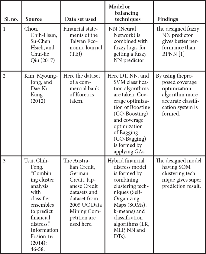
18
An Extensive Survey on the Prediction of Bankruptcy
Sasmita Manjari Nayak and Minakhi Rout*
School of Computer Engineering, Kalinga Institute of Industrial Technology (Deemed to be) University, Bhubaneswar, India
Abstract
Prediction of bankruptcy is an active area for research which is associated with the state of insolvency where a company or a person is unable to repay the creditors the debt amount. Up to now so many statistical and machine learning based models have been introduced for bankruptcy prediction. The pre-processing phase is an important step to enhance the performance of the model. Thus, one needs to choose effective pre-processing techniques which can be more suitable for the data set considered. So, this chapter focused on both the model, specifically, ensemble models for classification to address how new improved models are developed by combining two or more simple developed techniques and pre-processing techniques in order to address the imbalanced nature of the data and outlier if any present in the data. In most of the chapters the authors make some comparisons to show up the performance of their models with some other previously developed models. Here, we observed from the survey that the pre-processed datasets give better prediction outcome and it also proved that the ensemble models are more powerful for bankruptcy prediction as compared to the single models.
Keywords: Bankruptcy prediction, ensemble models, imbalance dataset, outlier, pre-processing, machine learning, oversampling, undersampling
18.1 Introduction
A company, having bond non-payment, overdrawn bank accounts, non-payment of bonus, or the announcement of bankruptcy, is taken as a failed company. The bankruptcy of a company hampering both the company’s goodwill, as well as shareholders benefits and therefore affects the economic growth of the company. To minimize these effects, the bankruptcy prediction (BP), would be necessary [1]. If a corporation is having higher stage of debts and such situation is going on for many years then that company becomes distressed. That means the company is unable or faces difficulty to pay off the debt, which leads to a bankruptcy situation. So, in some cases due to financial suffering or financial discomfort bankruptcy occurs. In some other cases firms suffer from bankruptcy just after facing a trouble, like a major fraud [16].
Different techniques are generally used to find out, the interrelation between bankruptcy of a company’s and its financial ratios like cash ratio, profitability, solvency, etc., known as a bankruptcy prediction model (BPM). By taking the facts at hand or by taking present information of a company the BPM is constructed, assuming that such relationship occurs in the future means that model can be used in future for prediction of bankruptcy. The performance of BPM is not only dependent on which types of financial ratios are selected and which techniques are used, but it is also depended on type of data that is taken for that model [2]. For choosing the dataset, one of the simplest methods is to use all data present at hand but when considered about a dataset having huge number of data, it becomes non-successful only because of high computing time and space. Another type of simple sampling technique is random sampling. When datasets have less number of data, there cannot be such types of problems like computing time and space. The fact remains that the number of bankrupt companies is very few as compared to non-bankrupt ones, for which an imbalanced problem arises. Without doing any procedure for balancing the imbalanced dataset, one cannot get accurate performance in classification, whatever may be the sampling strategy.
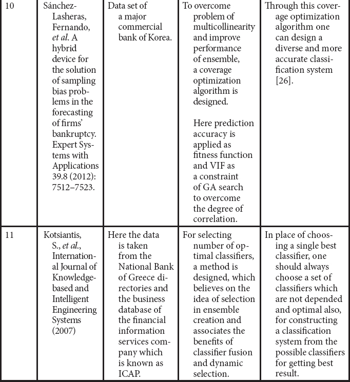
At the time of forecasting of bankruptcy the imbalance property of the datasets is ignored by some authors. But actually, the degree of imbalance or inequality which is the ratio of number of bankrupt to non-bankrupt may be nearby equal to 1 to 100 or even 1 to 1,000. So the imbalance problem should be discussed in bankruptcy prediction [2]. There are mainly two identified issues in imbalance datasets. The first is when a BPM uses a dataset which has very less number of bankrupt firms. In such situations, for bankrupt firms, the performance of BPM is diminished. The second is handling imbalanced datasets and enhancing the performance of the BPM [13].
An outlier can be defined as an outside data in a dataset or data having completely dissimilar character from others in a dataset, with basis on some measurement. An outlier data always contains useful information related to that dataset [14]. So handling of outliers should be done very carefully. Outliers can be handled either by omitting the outlier data or by winsorization. Omission i.e. deletion of outlier data from dataset is not preferable always as outliers are also part of reality [7]. Before handling of outliers, detection of outlier should be done. Outliers may be detected by setting a threshold value. After handling the outliers in a dataset the accuracy of BPM increases as the bad data or the outliers are removed from the dataset [9].
By using ensemble learning the predictive capability of single classifiers can be improved and simultaneously error is also reduced. Through ensemble learning we can get a strong classifier i.e. a highly accurate classifier by combining number of weak classifiers [15]. By combining multiple classifiers ensembled classifier is constructed [16]. Three things should be considered before construction of an ensembled classifier. At first one should consider which classifiers have to be taken from the available classifiers. Secondly how many classifiers are taken and the most important point is that which technique should be taken for constructing the ensembled model [17].
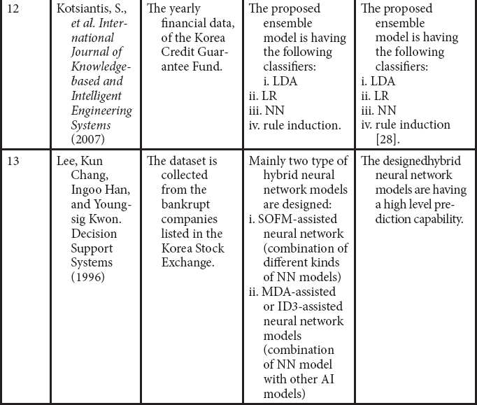
18.2 Literature Survey
18.2.1 Data Pre-Processing
Preprocessing of data can be said as a technique through which the data of a dataset can be given a useable form. For this purpose there are at present several techniques through which the classification accuracy can be improved [8]. Balancing the imbalance dataset, handling the outlier mainly comes under data preprocessing.
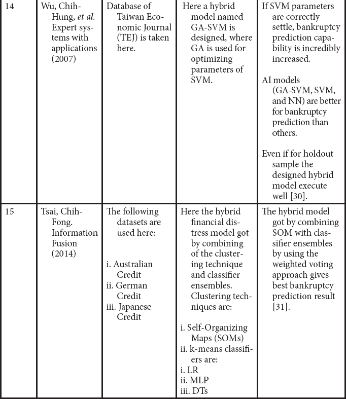
18.2.1.1 Balancing of Imbalanced Dataset
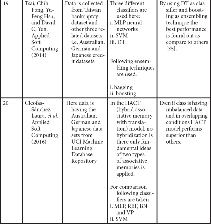
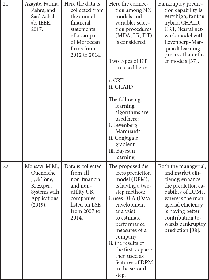
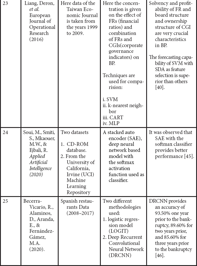
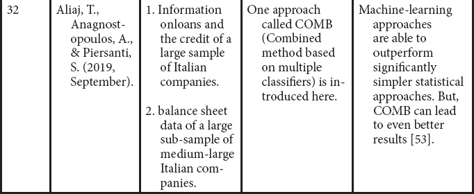
A dataset is called imbalanced when it is having unequal distributions or in other word it can be said, a dataset is imbalanced when one class is having absolutely different numbers than another [13]. Imbalance problem arises when all most all data are associated with the majority class. Mainly due to the imbalance problem the predicting capability of BPM deteriorates [10]. Practically as compared to non-bankrupt cases, the bankrupt cases are extremely less. So, it can be said that the numeral value of bankrupt cases as compared to non-bankrupt cases is nearly equal to zero. That’s why severely imbalanced problem arises. So for a dataset first balancing is necessary before classification.
Through the review we get that the BP rate is high for balance dataset as compared to imbalance dataset for the same classifier. To balance the datasets the authors go through the following balancing techniques. Presently there are mainly two principal types of balancing techniques: one is oversampling and another is undersampling. In oversampling sampling is done in the minority class over and over that means again and again new data are added in minority class, whereas in an undersampling a part of the majority class is selected for getting same numbered samples in both classes. Both oversampling and undersampling are called resampling. The work, which were already reported on the imbalance factor of data and the techniques used to handle it are discussed in Table 18.1.
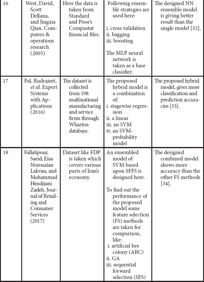
18.2.1.1.1 Oversampling
There are presently a number of oversampling techniques. Through review we get the following oversampling methods.
- Random Oversampling with Replication (ROWR):
Here some instances are chosen from the minority class, then replicated them again and again then after they are added into the same minority class. This procedure is continued until both the classes are having equal number of instances. - Synthetic-Minority-Over-sampling-Technique (SMOTE): One of the. advanced oversampling methods. of ROWD is SMOTE, where oversampling of minority class takes place through the synthesized data not through replicated data as ROWD. In SMOTE data is synthesized by taking each minority class data and then the synthesized data is placed anywhere on the line joining the point under consideration and its chosen neighbor among its k nearest neighbors [2].
- Borderline-SMOTE (BSMOTE):
In BSMOTE synthetic data is produced only for those data which are presently on borderline of minority class but not for all. Here first the data which are present on borderline are found out from the original dataset and after that new data are synthesized for them. Then those new data are combined with the master dataset.
18.2.1.1.2 Undersampling
As oversampling, there are also presently a number of undersampling techniques. Through review we get the following undersampling methods.
- Random Under-sampling (RU):
In random under-sampling method the imbalanced classes are balanced by eliminating data from the majority class. This procedure is continued till both the majority and minority class instances are balanced out.Table 18.1 Findings from different chapters working on imbalance data through review.
Chapter Dataset Balancing strategies Classifiers Outcome Future work 1 Zhou, L. (2013). - USA Bankruptcy Dataset (USABD)
- Japanese Bankruptcy Dataset (JPNBD)
ROWR, SMOTE, RU, UBOCFNN, UBOCFGMD. LDA, LOGR, C4.5 (DT), NN and SVM Sampling method depends on number of bankrupt cases. For few numbers of bankrupt cases, oversampling method SMOTE is used, but if there are presently huge number of bankruptcy cases, the combination of SMOTE and undersampling method may be used. Identification of difficult and easy observations for testing, as training sample and bankruptcy prediction models [2]. 2 Kim, T., & Ahn, H. (2015). H Bank’s bankruptcy data for non-externally audited companies in Korea. By combining k-RNN and OCSVM, new hybrid under-sampling method is introduced. LR, DA, CART and SVM Whatever may be the sampling method, here SVM shows better prediction result.
Performance of LR, DA, and CART is improved by applying this hybrid approach, as compared to simple random under-sampling.- To optimize the parameters of this hybrid method a mechanism should be found out.
- Some more sampling methods have to be tested [3].
3 Kim, H. J., Jo, N. O., & Shin, K. S. (2016). Dataset having 22,500 small- and medium-sized Korean manufacturing firms CBEUS method is used Hybrid model that combines the Genetic Algorithms (GA) and the Artificial Neural Networks model (GA-ANN) are introduced. The performance of GA-ANN with cluster-based evolutionary under sampling was superior than ANN with random sampling, GA-ANN with random sampling, and GA-ANN with evolutionary sampling. Clustering algorithms, such as self-organizing maps, and hierarchical agglomerative clustering should be tested in future [4]. 4 Sisodia, D. S., & Verma, U. (2018). The Spanish bankruptcy dataset which is collected from GitHub is used here Oversampling methods like SMOTE, BSMOTE, SLS, and ROS and undersampling methods like RUS and CNN are used here. Three individual classifiers i.e. C4.5, LR, and SVM and three ensembled classifiers i.e. AdaboostM, DTBagging, and RF are used here. Here no one is the best for all but for oversampling LR and DTBagging are better where as for undersampling C4.5 and RF are better.
Here oversampling method with DTBagging gives best prediction result as compare to others [5].5 Le, T., Le Son, H., Vo, M. T., Lee, M. Y., & Baik, S. W. (2018). Korean bankruptcy dataset (KBD). Here the undersampling method is used, in which IHT (Instance Hardness Threshold) concept is used to remove noise. The Cluster-based boosting (CBoost) classifier is used. The Robust Framework using the CBoost algorithm and IHT(RFCI) performs better than the GMBoost algorithm, the oversampling-based methods, and the clustering-based undersampling method. To find out a cost-sensitive method which can deals with the class imbalance problem in order to get an optimized model to predict bankruptcy [6]. 6 Kim, M.J., Kang, D.K., & Kim, H.B. (2015). Dataset of Korean commercial bank is used here. Here SMOTE technique is used to balance the data. Here following techniques are used for classification: - SMOTEBoost
- SMOTE-CostBoost (the combination of CostBoost and SMOTE)
- SMOTE-GMBoost (the combination of GMBoost with SMOTE)
For both imbalanced data and balanced data, GMBoost has the highest prediction power than the other. For multiclass classification problem, where severe imbalance problem are found, GMBoost algorithm can be applied there [10]. 7 Vieira, A.S., Ribeiro, B., Mukkamala, S., Neves, J.C., & Sung, A.H. (2004). A financial data having 780,000 financial statements of French companies Two types of companies are considered: - bankrupted companies misclassified as healthy
- companies misclassified as bankrupted.
Three classifiers like linear genetic programming (LGP), support vector machines and artificial neural networks (ANN) are considered. LGP shows best prediction for the balanced dataset but for the imbalanced dataset it’s prediction power is not so good.
HLVQ and SVMs are perform best for the imbalanced datasetsSome financial ratios can have large annual variation, so as a future work the records of these ratios from a longer period should be taken [20]. 8 Wang, M., Zheng, X., Zhu, M., & Hu, Z. (2016, November) The data is collected from the website Wangdaizhijia (http://www.wangdaizhijia.com/), which handles a Chinese P2P online lending portal. Here SMOTE algorithm is used to solve the imbalance problem Four classifiers are used - Logistic Regression
- Artificial Neural Network
- SVM
- Fuzzy SVM)
A new model FSVM-RI is designed, which uses fuzzy SVM as classifier with region information for BP.
The designed model used fuzzy membership function for which, it decreases the effect of outliers.
It is having higher prediction rate, even if there is present outliers and missing values in the database.The statements of financial expertise should be included for prediction and some more datasets should be included to measure the accuracy of the prediction [41]. 9 Smiti, S., & Soui, M. (2020). Datasets are obtained from the University of California, Irvine (UCI) Machine Learning Repository (https//archive.ics.uci.edu/ml/datasets.html). Apply Borderline SMOTE as a data preprocessing method to balance the original data set. Softmax classifier BSM-SAES approach, which combines Borderline Synthetic Minority oversampling technique (BSM) and Stacked AutoEncoder (SAE) based on the Soft-max classifier outperforms the other’s applied methods. To enhance the AUC of the bankruptcy prediction model by using a comprehensible evaluation model based on IF-THEN rules [54]. 10 Sun, J., Li, H., Fujita, H., Fu, B., & Ai, W. (2020). Based on the sample data of Chinese public companies listed in Shanghai Stock Exchange and Shenzhen Stock Exchange. Uses SMOTE Two class-imbalanced DFDP models based on Adaboost-SVM ensemble combined with SMOTE and time weighting
1. S-SMOTE-ADASVM-TW
2. E-SMOTE-ADASVM-TWThe E-SMOTE-ADASVM-TW model significantly outperforms the S-SMOTE-ADASVM-TW model and is more preferred for class-imbalanced DFDP. These two models can be further applied to solving the other problems such as default diagnosis, customer classification, spam filtering, etc. [55]. 11 Shrivastava, S., Jeyanthi, P.M., & Singh, S. (2020). Data collected for failed and survived public and private sector (2000–2017) 1. SMOTE is used to convert imbalanced data in a balanced form.
2. Lasso regression is used to reduce the redundant features from the failure predictive model.To avoid the bias and over-fitting in the models, random forest and AdaBoost techniques are used and compared with the logistic regression. AdaBoost gives the maximum accuracy in comparison to all other methods [56]. - Undersampling Based on Clustering from Nearest Neighbor (UBOCFNN):
In this sampling technique first the dataset should be divided into K number of clusters and points those are nearest to the data present at the centre of each cluster represents entire cluster. - Undersampling-Based on-Clustering from- Gaussian-Mixture-Distribution (UBOCFGMD): Conceptwise. this undersampling technique looks almost the same as that of UBOCFNN. There is presently only one difference that is clustering of UBOCFGMD occurs on the basis of Gaussian mixture distribution [2].
- Cluster-based evolutionary undersampling (CBEUS) Through this balancing technique the imbalance problem of data can be eradicated by combining clustering and genetic algorithm (GA) [4].
- Undersampling Approach Using IHT
Here Instance Hardness (IH) property is used to indicate the probability of a data being misclassified. Those data points which are present on the borderline of two or more classes have high IH values. In Undersampling Approach Using IHT, the data having high IH values is removed from majority class until got the balance [6].
18.2.1.2 Outlier Data Handling
The outlier is a data of a database, which lies far away from the rest of the values, or in other words it can be said that outlier is nothing but an extreme value. Before handling the outliers they should be identified or detected first. Several approaches are found for identifying and handling outlier.
18.2.1.2.1 Outlier Detection
Through review we get the following outlier detection methods.
- Distribution-based outlier detection:
On basis of statistics, such type of detection technology is designed. First of all, by taking the required dataset, statistical models are developed. Those data which have very less possibility having in statistical model, are taken as outlier data. - Distance-based outlier detection:
In this method through kth-Nearest Neighbor (kNN), outlier is detected. Here, the distance from an object to its kth nearest neighbor is measured. If the neighboring points of a data are comparatively close, then that data is taken as a normal data. But if the neighboring points are not close that means they are far away, then that data is taken as an outlier. - Density-based outlier detection:
Herein outlier is. detected depending on density of data in a definite region. Here a data which is present in the low density regions is taken as an outlier. - Distance-based clustering approach:
Such method, first distributed the whole dataset in two subgroups, as bankrupt and non-bankrupt. Then, k-means clustering approach is applied to obtain two cluster centers, denoted by C1 and C2 for the two subgroups. After that the Euclidean distance measure is applied to obtain the distance in between C1 and C2 and each data point in the subset is calculated. The data points which are at a longest distance from cluster centers are taken as outliers [9]. - k-Reverse Nearest Neighbor (k-RNN):
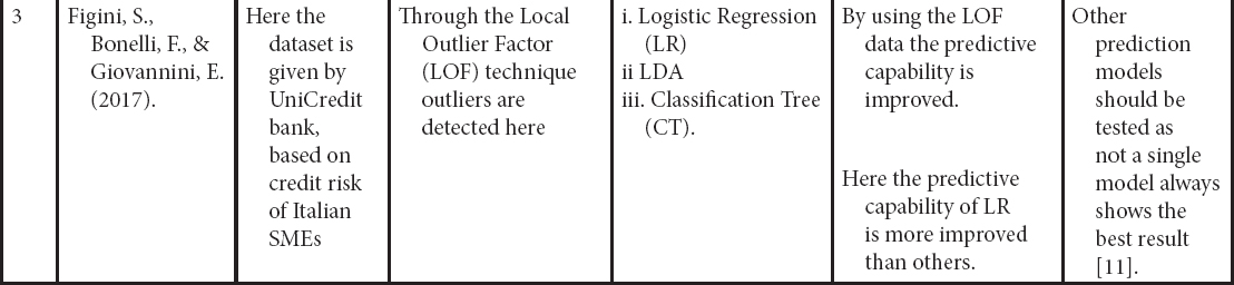
To identify the outliers, the concept of the k-NN is used here. In kth-Nearest Neighbor (k-NN), for each data of the dataset there must be present at least k nearest neighbors, where k is any natural number. But in k-RNN, there is no certainty about the presence of the reverse neighbors. For example, when a data in the dataset is far away from other data points, there is no element present in its k-RNN. Or we can explain it as, if a data has many k-RNNs, it means it has a number of neighbors. So that data has very least possibility to be an outlier [3]. - Local Outlier Factor technique (LOF):
In this outlier detection method local density (LD) of a data, which is defined by considering the K-NN, is considered. Here comparison takes place between LD of a data and its nearest neighbors. When LD of that data is having non-identical value as compared to its neighbors, then that data of the dataset is taken an outlier [11]. - Standardization and Percentiles:
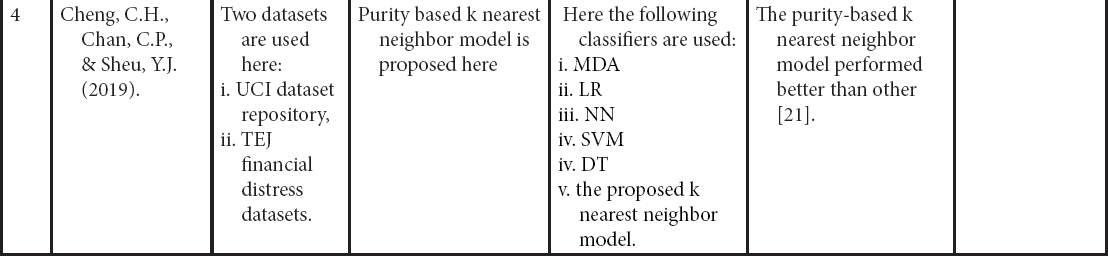
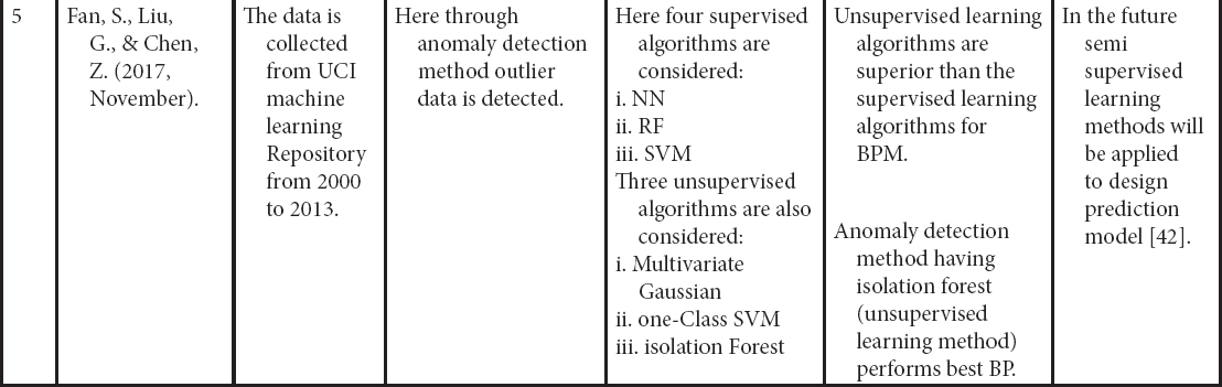
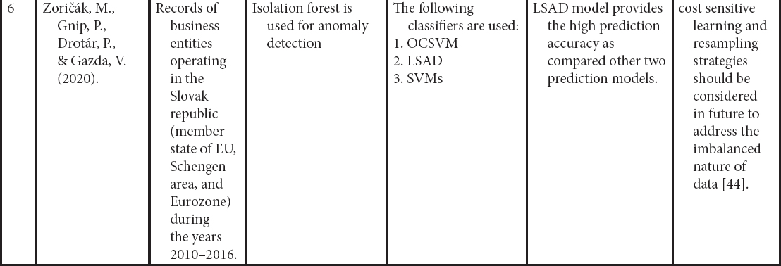
Here, one or more values are taken as threshold. Through that threshold value an outlier is detected. Data value which comes beyond the threshold value is taken as an outlier [7].Table 18.2 Findings from different chapters working on outlier data through review.


- Multivariate Gaussian distribution:
By using this method the outlier is detected, on basis of the interconnection impact among features of a database. Here the probability of a data point as central point is calculated. The data point having low probability is taken as an outlier [44]. - Isolation Forest (IF):
It is an unsupervised and non-parametric formulation to anomaly detection. It attempt to isolate anomalies in data instead of using anydistance or density formulae. The IF builds the ensemble of isolation trees. The data samples which are having the short average length on these isolation trees are considered as anomalies.
18.2.1.2.2 Outlier Handling
Handling of outlier should be done after its detection. Deletion or winsorization are mainly the two things which can be done for handling outliers. They may be the extreme values but deletion of data cannot be taken as an appropriate approach for handling outliers, as they are also part of the dataset. Outliers are more important when there are present limited numbers of observations, for which they should not be omitted from the dataset. But they must go through proper preprocessing before utilization.
For preprocessing or handling outlier, winsorization is an appropriate method. In this technique after detection of an outlier, without omitting that should be replaced with a very nearest value of it. It may be possible that after removing an outlier by its “nearest neighbor” that may still be detected as an outlier. To overcome such type of problem “dynamic” winsorization is applied. In dynamic winsorization, after substituting nearest neighbor as an outlier, again it is detected whether that new value is an outlier or not. If it is found that the new substituted value is an outlier then, that value is again substituted by its nearest neighbor. This procedure should be repeated up to the outliers comes under the threshold value set previously. The work based on above problem of outlier and the techniques to handled it are discussed in Table 18.2.
18.2.2 Classifiers
Literally classification means categorizing of a collection of items into different groups. Assignment of different data items of a dataset into different classes is called classification. Actually through classification one can find the exact categories of the data items of a dataset. The functions which are used for classification of dataset in data mining are known as classifiers.
Through review we get the following classifiers.
- Support vector machines (SVM):
In SVM data is classified through optimal hyperplane. Here input vectors are mapped onto an N-dimensional. attribute space which builds the optimal .hyperplane. The optimal hyperplane divides the training examples into two groups, i.e. data points far away from the hyperplane and the nearest to the hyperplane. Support vectors are the data which are nearest to optimal hyperplane [3]. - Fuzzy SVM:
Fuzzy SVM gives emphasis on outliers as well as on noises, as in real datasets, most of the time, some outliers or noises are remain present, which affect the accuracy of the classifiers. Fuzzy SVM mentioned a fuzzy membership function 0 ≤ xi ≤ 1, that is linked with each data xi. xi shows the position of the consequent instance xi with regard to a class. - SVM+:
SVM+ takes some more extra information about learning. It is designed for taking benefits of the structure of data, like region information. - FSVM-RI (Fuzzy SVM with region information):
FSVM-RI is the combination of both Fuzzy SVM and SVM+. So it takes advantages of both the models, for which it has more confined limitations than SVM+. It can reduce the impact of outliers as well as use the group information [41]. - One-class Support Vector Machine (OCSVM):
OCSVM is different from SVM. It works with training data having one class only. In OCSVM through support vectors one can describe the data from a single class. It is possible to separate a class from rest of the feature by a boundary in OCSVM. Always it is preferable to use OCSVM in place of SVM [3]. - Multilayer perceptron (MLP):
MLP is a network having three layers of computational nodes i.e. an input layer for inputting the value, an output layer for getting output, a value in between 0 to 1and just a single or many hidden layers may remain in between them for taking the input signals and converts them into an output as for requirement. Here a weight is connected with each interconnection which can be adjusted during the training phase. - Logistic regression (LR):
Through LR the existence of an incident can be estimated. For which data is placed on logistic curve. Value. of two. Class. Labels. shows yes/no and sequential .variables shows result of variables- i.e., low, medium- or -high are calculated by LR. - C4.5 decision trees (DT):
This decision tree is constructed on basis of C4.5 algorithm. In each DT every -internal .node shows a -test on a feature, whereas every branch shows result of a test. Classes are represented as the leaf nodes. The root is having the highest information, then an attribute from rest attributes having maximum information is taken as next node [9]. - CRT (Classification and regression tree):
The CRT algorithm divide data into two groups for making each group more homogeneous than before. The groups are again and again divided up to the conditions for homogeneous are satisfied. - CHAID (Chi-squared automatic interaction detector):
CHAID is used to find out the link among variables. It is mainly used for tree construction, which is based on the chi-square algorithm. It is not a binary tree as here at any level in the tree model, can produce more than two [37]. - Linear discriminant analysis (LDA):
In linear discriminant analysis discrimination score or z-score is produced for identifying two groups by adding descriptive variables to a linear -function. Where z-score can be calculated like where xi stands for explanatory variables, wi is the discriminant weights, c is a constant.
 - Neural networks:
The neural networks technique imitates the working technique of a human brain. Here a functional mapping of input variables takes place with output variables [13]. - Radial Basis Function (RBF):
RBF uses only one single hidden layer for classification not as MLP which may use number of hidden layer. In the training stage RBF uses Gaussian function like activation functions whereas least-square criterion like .objective functions. Except hidden layer there is an input layer, as well as an output layer. - Ant-miner-algorithm-for-classification rule-induction (CRI): On basis of a probability function the ants choose the feasible path in CRI. Here feedback mechanism is used. Path having huge amount of pheromone as well as heuristic value, is selected by ants, after visiting all possible paths [43].
- The Tobit model:
Through the censored regression models auxiliary data of majority class is combined with the binary data. This model is based on censoring technique, which is used for censored data as well as data present on the borders. - The Grabit model:
An extension of Tobit model is Grabit model. Here gradient boosting with trees is used as base learners. This is a very flexible approach due to boosting with trees [19]. - Linear Genetic Programming (LGP):
In LGP, Genetic Programming (GP) technique is used. Machine code level management and estimation of .programs takes place in this technique [11]. - Weighted-vote Relational Neighbor (wvRN) classifier:
In wvRN classifier, the bankruptcy probabilities is depended on the boundary values. Boundary value of a node may be one or zero, which depends on neighbor’s bankrupt situation. - Multivariate discriminant analysis:
The Fisher procedure is applied, for which a discriminant function is used in the Multivariate discriminant analysis method. Ratio of between-groups with within-groups variances is maximized for constructing a discriminant function. - ID3:
In the ID3 a decision tree is generated, which classifies the training sample with the help of the entropy measure. Here no need of constructing a decision rule as a discriminant function [29]. - Cerebellar model neural network (CMNN):
This is one of the learning mechanisms which imitates cerebellum of human being. In the training stage, the cerebellar model neural network becomes expert in analysis of financial statement, further which is used for forecasting of bankruptcy [39]. - Least-Squares Anomaly Detection (LSAD):
The LSAD is similar to OCSVM, however it uses different loss function that makes it easier and quicker to train without compromising the prediction performance. LSAD is extended form of the least squares probabilistic classification [44].
18.2.3 Ensemble Models
Ensemble models are made by combining several simple single models. By this approach one can get better bankruptcy prediction result as compared to single models. Through review we got the following ensemble techniques.
- Boosting tree:
Boosting is an additive technique. In boosting ensemble technique a new model is inserted to the existing one for reducing errors of the previous models. Here models are added one after another till further improvement is impossible [8]. - AdaBoost algorithm:
AdaBoost is a boosting algorithms, which can be used for imbalanced dataset. AdaBoost is more robust than boosting algorithm as AdaBoost overcomes the problems of boosting algorithm like the over-fitting and generalization problem. - AdaBoostM1:
Through the AdaBoostM1 boosting technique can be improved. It is an iterative process and by this process data subsets are created for the base classifier, for which resampling of the training data sample is done [12]. - Random Forest (RF):
In Random Forest decision trees are ensemble which is otherwise called as random subspace. A huge number of individual decision trees are taken for outputting the required class in training stage [5]. - Geometric mean based boosting (GMBoost):
Geometric mean based boosting can be applied on imbalance dataset. It is the modification of AdaBoost algorithm. The only difference is that GMBoost applies geometric error in place of arithmetic-error-of AdaBoost.Table 18.3 Findings from different chapters working on ensembling methods through review.


- Cost-sensitive boosting:
In this boosting algorithms, for the misclassified instances penalty is assigned from minority class [10]. - Cluster-Based Boosting (CBoost):
CBoost algorithm is the modification of the AdaBoost algorithm. Here to handle the class imbalance problem, initial weight is customized for every data with the help of k-mean clustering algorithm [6]. - BAGGING-:
In the Bag technique multiple sets of input data will be generated with replacement by sampling the input data. Then for each set classifier is built and finally the classifications are combined using a majority voting policy. - Random subspace (RSP):
In RSP method, the base classifiers are trained on sets, which are taken randomly from the master dataset. Then results of each classifier are combined for getting rule by a simple majority voting method. - Rotation forest (RotF):
In Rotation forest the feature set is divided into number of subsets randomly. Then on each subset Principal Component Analysis (PCA) is applied. After that by pooling all principal components a set of variables is newly formed then data is changed according to the newly created feature space. At last training of the main classifier takes place by taking the newly created dataset. - DECOR:
In this algorithm a base learner is used for constructing an ensemble classifier by repeatedly combining distinct arbitrary produced classifiers with the training set. - MDA-assisted-neural-network:
This neural network model is used as a preprocessing mechanism. MDA (mean decrease in accuracy) method is used where important input variables are selected. Those later may be utilized in NN model. - ID3-assisted-neural-network:
In this type of neural -network, ID3 is used as preprocessing mechanism. Input variables are selected through ID3 which will be applied in the neural network model. - SOFM-assisted-neural-network:
This type of neural network is the result of fusing two models i.e. SOFM and LVQ (Linear Vector Quantization), to extract more refined clusters from the given input dataset [29]. - Max voting (MV):
In the MV technique, many single classifier models are employed to decide on every data-point and the output of every individual single classifier is considered as a ‘vote’. The final output (decision) is based on the majority’s answer. - Averaging:
The averaging technique is very similar to the MV technique; however, an average of the outputs of all individual or single classifiers represents the final output (decision). However, unlike the MV, the averaging technique can be used for both regression and classification machine learning task. - Weighted average (WA):
The WA is an expansion to the averaging techniques. In this technique, weights are assigned to each and every model to indicate the importance of an individual model for the prediction. - Stacking (STK):
It perform predictions from several models (m1, m2,…, mn) to build a new prediction model, where as the new model is made use of test data set for predictions. It tries to increase the predictive power of a classifier. - Blending (BLD):
The blending ensemble approach is similar to stacking but the difference is stacking uses test data set for prediction where as blending uses a holdout validation method from the training data set for predictions [47].
18.3 System Architecture and Simulation Results
The process of construction of a bankruptcy prediction model can be represented pictorially as follows:
The steps specified in Figure 18.1 is the general framework to be followed whenever we for bankruptcy prediction.
To prove that the ensemble model is performing better than a single classifier which is also proved in many of the published work by different authors in the reviews. We have also applied some of the ensemble models on the bankruptcy data set collected from www.kaggel.com. The outcome of the simulation results is listed in the form bar chart, RoC curve from Figure 18.2 to 18.7. From the plots and figures, we observed that the claim that many authors has made on ensembles model is true.
18.4 Conclusion
Through this review we surveyed on different preprocessing techniques as well as ensembling techniques. Here it is found that for the proper prediction of bankruptcy one should first give emphasis on preprocessing of dataset i.e., balancing of imbalance dataset and detecting and handling of outliers from the dataset. Type of sampling technique based on numeral value of bankrupt cases (BCs). When there are a small number of BCs present, the oversampling technique SMOTE may be considered, but when there are enormous numbers of BCs present, both SMOTE and some undersampling technique give better result [2]. A particular sampling technique can’t give the best result for the entire set of classifiers. When oversampling technique is considered LR and DTBagging classifiers may be taken for better result likewise for undersampling technique C4.5 and RF classifiers may be taken [5]. Whether data may be balanced or imbalanced, GMBoost has the highest BP capability than others [10], but the RFCI achieves better prediction result than GMBoost, oversampling techniques, and undersampling techniques based on clustering [6]. One of the hybrid under-sampling techniques which is constructed by combination of the k-RNN and OCSVM increases the rate of correctness of classifiers, like LR, LDA, DT, SVM, etc. [3]. GA-ANN with CBEUS gives better prediction result than ANN with ROWR or RU, GA-ANN with ROWR or RU, and GA-ANN with CBEUS [4]. LGP shows the best BP capability when used for the balanced data, whereas HLVQ and SVM are best for the imbalanced data [20].
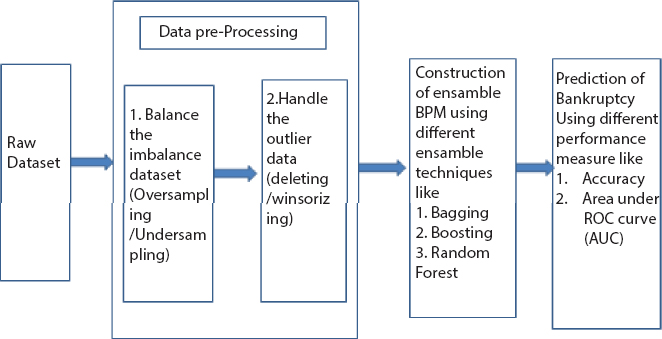
Figure 18.1 Architecture of a bankruptcy prediction model.
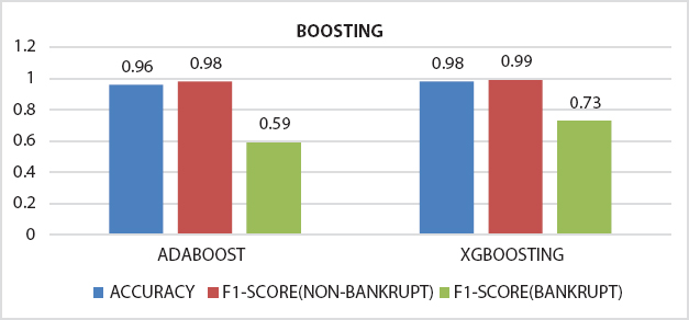
Figure 18.2 Comparison of accuracy and F1-score obtained from Adaboost and XGBoosting.
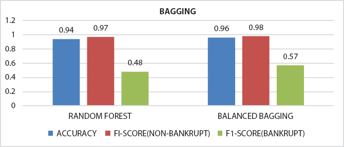
Figure 18.3 Comparison of accuracy and F1-score obtained from bagging based models.
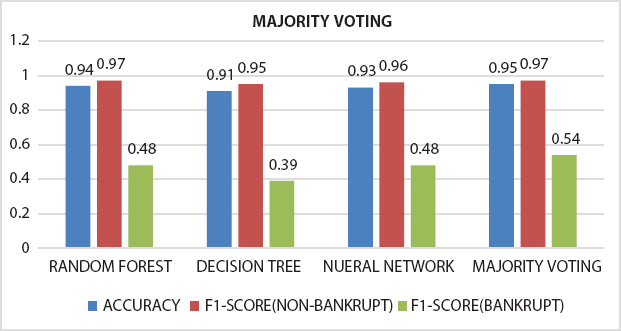
Figure 18.4 Comparison of accuracy and F1-score obtained from single classifier (DT and NN) and ensemble model (RF, MV).
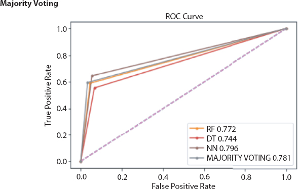
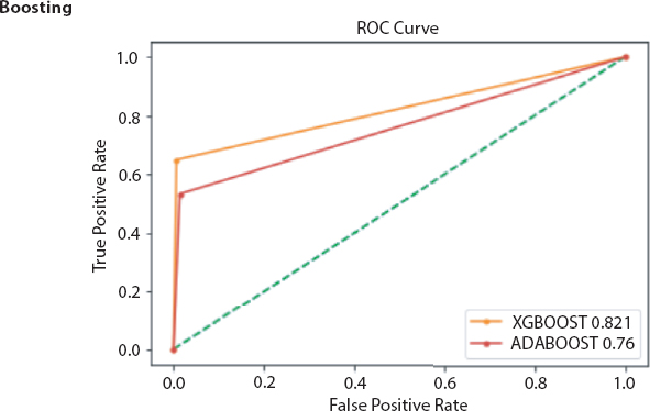
Figure 18.6 RoC curve obtained from boosting based ensemble models.
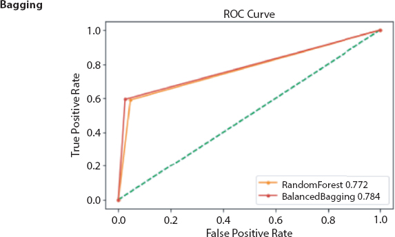
Figure 18.7 RoC curve obtained from bagging based ensemble models.
When we consider about the outliers the BP capability of FSVM-RI model is very high, even though the database is having outliers and missing values [41]. When outliers are there in the dataset decision trees can give highest prediction result as compare to others [7]. By removing 50% of the outliers, prediction capability can be optimized for SVM, ANN, and LRDT. Here SVM gives the highest BP rate than others [9]. Through LOF technique BP power can be improved. By applying LOF the predictive capability of LR is more improved than LDA and CT [11]. Anomaly outlier detection method has isolation forest (unsupervised learning method) that performs best BP [42].
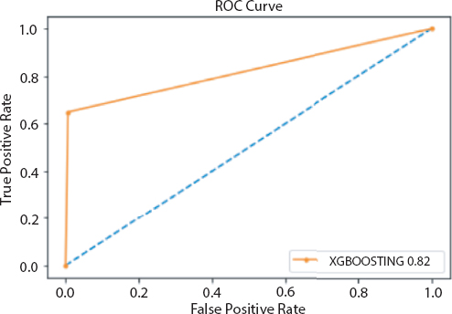
Figure 18.8 Roc curve obtained from XGBoosting model.
After preprocessing of dataset classifiers are made for making bankruptcy prediction models. In place of choosing a single best classifier, one should always choose a set of classifiers which are not dependent and optimal also, for constructing a classification system from the possible classifiers for getting best result [27]. Here it is found that ensembling classifiers which are made by combining number of classifiers with the help of different ensembling methods are always superior to the single classifiers on basis of prediction rate. The predictive power of an ensemble model is basically controlled by types of data available in a dataset [22]. From the serve we get the following ensembled models like Fuzzy NN predictor, Hybrid financial distress model having SOM clustering technique, XGBS, gXGBS and gXGBS_hist, Grabit model, SOFM-assisted NN model and MDA-assisted NN models, etc., which are mentioned above in Table 18.3. From the above survey it is found that the prediction power of XGBS, gXGBS and gXGBS_hist is extremely good for all types of data i.e. data may be balanced or imbalanced [18]. When the sample sizes are smaller, the predictive capability of the Grabit model is larger, whereas for the sample having largest size, the predictive power is almost same as boosted Logit model [19]. The ensemble model constructed by the combination of MDA, LR, CRT, ANN and AdaBoost methodology is having 88.8% of accurate [24]. Even if class is having imbalanced data and in overlapping conditions HACT model performs and is superior to others [36]. Result obtained through different classifiers are pictorially represented in Figures 18.1 to 18.8.
So for getting a perfect or best model for prediction of bankruptcy one has to first preprocess the data for getting proper dataset. Then by taking a proper ensembling technique an ensembling model should be developed.
References
1. Chou, C.-H., Hsieh, S.-C., Qiu, C.-J., Hybrid genetic algorithm and fuzzy clustering for bankruptcy prediction. Appl. Soft Comput., 56, 298–316, 2017.
2. Zhou, L., Performance of corporate bankruptcy prediction models on imbalanced dataset: The effect of sampling methods. Knowledge-Based Syst., 41, 16–25, 2013.
3. Kim, T. and Ahn, H., A hybrid under-sampling approach for better bankruptcy prediction. ![]() (Intelligence Research), 21, 2, 173–190, 2015.
(Intelligence Research), 21, 2, 173–190, 2015.
4. Kim, H.-J., Jo, N.-O., Shin, K.-S., Optimization of cluster-based evolutionary undersampling for the artificial neural networks in corporate bankruptcy prediction. Expert Syst. Appl., 59, 226–234, 2016.
5. Sisodia, D.S. and Verma, U., The Impact of Data Re-Sampling on Learning Performance of Class Imbalanced Bankruptcy Prediction Models. Int. J. Electr. Eng. Inform., 10, 3, 433–446, 2018.
6. Le, T. et al., A cluster-based boosting algorithm for bankruptcy prediction in a highly imbalanced dataset. Symmetry, 10, 7, 250, 2018.
7. Nyitrai, T. and Virág, M., The effects of handling outliers on the performance of bankruptcy prediction models. Socio-Econ. Plann. Sci., 67, 34–42, 2019.
8. Son, H. et al., Data analytic approach for bankruptcy prediction. Expert Syst. Appl., 138, 112816, 2019.
9. Tsai, C.-F. and Cheng, K.-C., Simple instance selection for bankruptcy prediction. Knowledge-Based Syst., 27, 333–342, 2012.
10. Kim, M.-J., Kang, D.-K., Kim, H.B., Geometric mean based boosting algorithm with over-sampling to resolve data imbalance problem for bankruptcy prediction. Expert Syst. Appl., 42, 3, 1074–1082, 2015.
11. Figini, S., Bonelli, F., Giovannini, E., Solvency prediction for small and medium enterprises in banking. Decis. Support Syst., 102, 91–97, 2017.
12. Zhou, L. and Lai, K.K., AdaBoost models for corporate bankruptcy prediction with missing data. Comput. Econ., 50, 1, 69–94, 2017.
13. Veganzones, D. and Séverin, E., An investigation of bankruptcy prediction in imbalanced datasets. Decis. Support Syst., 112, 111–124, 2018.
14. Aggarwal, C.C. and Yu, P.S., Outlier detection for high dimensional data. Proceedings of the 2001 ACM SIGMOD International Conference on Management of Data, 2001.
15. Kim, M.-J. and Kang, D.-K., Classifiers selection in ensembles using genetic algorithms for bankruptcy prediction. Expert Syst. Appl., 39, 10, 9308–9314, 2012.
16. Tsai, C.-F., Combining cluster analysis with classifier ensembles to predict financial distress. Inform. Fusion, 16, 46–58, 2014.
17. Tsai, C.-F., Hsu, Y.-F., Yen, D.C., A comparative study of classifier ensembles for bankruptcy prediction. Appl. Soft Comput., 24, 977–984, 2014.
18. Le, T. et al., A fast and accurate approach for bankruptcy forecasting using squared logistics loss with GPU-based extreme gradient boosting. Inf. Sci., 494, 294–310, 2019.
19. Sigrist, F. and Hirnschall, C., Grabit: Gradient tree-boosted Tobit models for default prediction. J. Bank. Financ., 102, 177–192, 2019.
20. Vieira, A.S. et al., On the performance of learning machines for bankruptcy detection. Second IEEE International Conference on Computational Cybernetics, 2004. ICCC 2004, IEEE, 2004.
21. Cheng, C.-H., Chan, C.-P., Sheu, Y.-J., A novel purity-based k nearest neighbors imputation method and its application in financial distress prediction. Eng. Appl. Artif. Intell., 81, 283–299, 2019.
22. García, V., Marqués, A.I., Salvador Sánchez, J., Exploring the synergetic effects of sample types on the performance of ensembles for credit risk and corporate bankruptcy prediction. Inform. Fusion, 47, 88–101, 2019.
23. Tobback, E. et al., Bankruptcy prediction for SMEs using relational data. Decis. Support Syst., 102, 69–81, 2017.
24. Fedorova, E., Gilenko, E., Dovzhenko, S., Bankruptcy prediction for Russian companies: Application of combined classifiers. Expert Syst. Appl., 40, 18, 7285–7293, 2013.
25. Sánchez-Lasheras, F. et al., A hybrid device for the solution of sampling bias problems in the forecasting of firms’ bankruptcy. Expert Syst. Appl., 39, 8, 7512–7523, 2012.
26. Kim, M.-J. and Kang, D.-K., Classifiers selection in ensembles using genetic algorithms for bankruptcy prediction. Expert Syst. Appl., 39, 10, 9308–9314, 2012.
27. Kotsiantis, S. et al., Selective costing voting for bankruptcy prediction. Int. J. Knowledge-Based Intell. Eng. Syst., 11, 2, 115–127, 2007.
28. Cho, S., Kim, J., Bae, J.K., An integrative model with subject weight based on neural network learning for bankruptcy prediction. Expert Syst. Appl., 36, 1, 403–410, 2009.
29. Lee, K.C., Han, I., Kwon, Y., Hybrid neural network models for bankruptcy predictions. Decis. Support Syst., 18, 1, 63–72, 1996.
30. Wu, C.-H. et al., A real-valued genetic algorithm to optimize the parameters of support vector machine for predicting bankruptcy. Expert Syst. Appl., 32, 2, 397–408, 2007.
31. Tsai, C.-F., Combining cluster analysis with classifier ensembles to predict financial distress. Inform. Fusion, 16, 46–58, 2014.
32. West, D., Dellana, S., Qian, J., Neural network ensemble strategies for financial decision applications. Comput. Oper. Res., 32, 10, 2543–2559, 2005.
33. Pal, R. et al., Business health characterization: A hybrid regression and support vector machine analysis. Expert Syst. Appl., 49, 48–59, 2016.
34. Fallahpour, S., Norouzian Lakvan, E., Zadeh, M.H., Using an ensemble classifier based on sequential floating forward selection for financial distress prediction problem. J. Retail. Consum. Serv., 34, 159–167, 2017.
35. Tsai, C.-F., Hsu, Y.-F., Yen, D.C., A comparative study of classifier ensembles for bankruptcy prediction. Appl. Soft Comput., 24, 977–984, 2014.
36. Cleofas-Sánchez, L. et al., Financial distress prediction using the hybrid associative memory with translation. Appl. Soft Comput., 44, 144–152, 2016.
37. Azayite, F.Z. and Achchab, S., The impact of payment delays on bankruptcy prediction: A comparative analysis of variables selection models and neural networks. 2017 3rd International Conference of Cloud Computing Technologies and Applications (CloudTech), IEEE, 2017.
38. Mousavi, M.M., Ouenniche, J., Tone, K., A comparative analysis of two-stage distress prediction models. Expert Syst. Appl., 119, 322–341, 2019.
39. Chung, C.-C. et al., Bankruptcy prediction using cerebellar model neural networks. Int. J. Fuzzy Syst., 18, 2, 160–167, 2016.
40. Liang, D. et al., Financial ratios and corporate governance indicators in bankruptcy prediction: A comprehensive study. Eur. J. Oper. Res., 252, 2, 561–572, 2016.
41. Wang, M. et al., P2P lending platforms bankruptcy prediction using fuzzy SVM with region information. 2016 IEEE 13th International Conference on e-Business Engineering (ICEBE), IEEE, 2016.
42. Fan, S., Liu, G., Chen, Z., Anomaly detection methods for bankruptcy prediction. 2017 4th International Conference on Systems and Informatics (ICSAI), IEEE, 2017.
43. Uthayakumar, J., Vengattaraman, T., Dhavachelvan, P., Swarm intelligence based classification rule induction (CRI) framework for qualitative and quantitative approach: An application of bankruptcy prediction and credit risk analysis. J. King Saud Univ.-Comput. Inf. Sci., 36, 2020, 647–657, 2017.
44. Zoričák, M., Gnip, P., Drotár, P., Gazda, V., Bankruptcy prediction for small-and medium-sized companies using severely imbalanced datasets. Econ. Model., 84, 165–176, 2020.
45. Soui, M., Smiti, S., Mkaouer, M.W., Ejbali, R., Bankruptcy Prediction Using Stacked Auto-Encoders. Appl. Artif. Intell., 34, 1, 80–100, 2020.
46. Becerra-Vicario, R., Alaminos, D., Aranda, E., Fernández-Gámez, M.A., Deep Recurrent Convolutional Neural Network for Bankruptcy Prediction: A Case of the Restaurant Industry. Sustainability, 12, 12, 5180, 2020.
47. Nti, I.K., Adekoya, A.F., Weyori, B.A., A comprehensive evaluation of ensemble learning for stock-market prediction. J. Big Data, 7, 1, 1–40, 2020.
48. Pisula, T., An Ensemble Classifier-Based Scoring Model for Predicting Bankruptcy of Polish Companies in the Podkarpackie Voivodeship. J. Risk Financ. Manage., 13, 2, 37, 2020.
49. Lahmiri, S., Bekiros, S., Giakoumelou, A., Bezzina, F., Performance assessment of ensemble learning systems in financial data classification. Intell. Syst. Account. Finance Manage., 27, 1, 3–9, 2020.
50. Lee, S., Bikash, K.C., Choeh, J.Y., Comparing performance of ensemble methods in predicting movie box office revenue. Heliyon, 6, 6, e04260, 2020.
51. du Jardin, P., Forecasting corporate failure using ensemble of self-organizing neural networks. Eur. J. Oper. Res., 288, 2021, 869–885, 2020.
52. Chen, Z., Chen, W., Shi, Y., Ensemble learning with label proportions for bankruptcy prediction. Expert Syst. Appl., 146, 113155, 2020.
53. Aliaj, T., Anagnostopoulos, A., Piersanti, S., Firms Default Prediction with Machine Learning, in: Workshop on Mining Data for Financial Applications, pp. 47–59, Springer, Cham, 2019, September.
54. Smiti, S. and Soui, M., Bankruptcy prediction using deep learning approach based on borderline SMOTE. Inform. Syst. Front., 22, 1–17, 2020.
55. Sun, J., Li, H., Fujita, H., Fu, B., Ai, W., Class-imbalanced dynamic financial distress prediction based on Adaboost-SVM ensemble combined with SMOTE and time weighting. Inform. Fusion, 54, 128–144, 2020.
56. Shrivastava, S., Jeyanthi, P.M., Singh, S., Failure prediction of Indian Banks using SMOTE, Lasso regression, bagging and boosting. Cogent Econ. Finance, 8, 1, 1729569, 2020.
*Corresponding author: [email protected]