
Chapter 1
Trendlines
Whether a trader is a practitioner of fundamental or of technical analysis, invariably, at one time or another, he has relied on trendlines to make his forecasts. Although trendlines are universally used, it is surprising how dissimilar they are in construction and interpretation, and how subjectively they are applied. Not only is it commonplace for different analysts to draw different trendlines representing the same data during the same time period, but the same individual, on separate occasions, will also draw two totally different trendlines based on the identical information, depending on his inclination each time. Consistency and uniformity are totally lacking. Not all the trendlines can be correct—only one is. Through exhaustive, painstaking research and years of experience and application, I have arrived at an effective method to select the two critical points that are essential to the proper construction of a trendline. Once learned and applied, trendline analysis is no longer subjective; instead, it becomes totally mechanical. Trendline breakouts are precisely defined and price objectives can be easily calculated: systems can actually be created. Price gaps and large price range moves assume a significance never before imagined.
Selection of TD Points™ and Construction of TD Lines™
Supply and demand dictate price movement. Specifically, should demand exceed supply, price advances; conversely, should supply exceed demand, price declines. These are basic economic tenets accepted by all economists. In order to illustrate this phenomenon pictorially, analysts construct a descending line to represent supply and an ascending line to represent demand (see Figures 1.1 and 1.2).
The difficulty, when creating these lines, involves the specific points to select and connect (see Figure 1.3). As it often does, human nature interferes in the proper construction of these lines. For example, we are accustomed to review the historical price activity of a market—from the past to the present, with the dates reading from left to right. As a result, the demand and supply lines are drawn and extended from the left side of the chart to the right. Intuitively, this is incorrect. Recent price activity is more significant than historical movement. In other words, precision and accuracy demand that the lines be extended from right to left, with the most recent date appearing at the right side of the chart. Initially, this may appear unorthodox but, in actuality, my experience and numerous observations confirm this approach. Simplicity and ease of construction should never serve as substitutes for logic and accuracy. Imprecision and total disregard for detail are reflected in the common practice of constructing multiple trendlines as well as in the typically cavalier attitude of analysts who believe that one of these lines will accurately define the trend. Success in using trendlines requires both an attention to detail and a pattern of consistency.
Source: Logical Information Machines, Inc. (LIM), Chicago, IL.
Figure 1.1 Note the declining price movement as defined by the downsloping “supply” line, as well as the pattern of both lower price highs and lows.
Source: Logical Information Machines, Inc. (LIM), Chicago, IL.
Figure 1.2 Observe the ascending price movement as depicted by the upsloping “demand” line as well as the series of both higher price highs and lows.
Source: Logical Information Machines, Inc. (LIM), Chicago, IL.
Figure 1.3 It's obvious that many lines can be drawn to establish the price trend. The key elements are to select the two critical points, construct the correct trendline, and ignore the many others.
Rather than merely presenting a set of rules designed to establish the proper method for selecting points and then connecting these points to construct a supply or a demand line, I would like to share with you a frustrating but professionally pivotal experience I had with a business colleague approximately 20 years ago. This episode proved to be a catalyst that changed my analytical life. Being fledgling traders, both he and I were consumed by the activity of the markets. Not only was the analysis of price behavior our profession, but it had also become our total obsession. Subsequent to leaving the office and returning home, we would preoccupy our evenings discussing interesting chart price patterns over the telephone. On one such occasion, we discussed at length the interplay of a series of price trends. We each drew the trendlines on our own charts. When we arrived in the office the next day and compared our respective charts, however, the lines on the charts did not even come close to resembling one another. This bothered me greatly. It was as if we had been speaking two entirely different languages to one another. I was determined to prevent this from ever happening again. It was essential that we both understood and communicated with the same vocabulary and definitions in order to avoid any further confusion and misunderstanding. Specifically, I embarked on a journey to catalog and standardize widely used market timing techniques, to improve on them, and to create my own. To this day, I strive to accomplish this goal. Trendlines were my first project.
For purposes of discussion and illustration, I will generally refer to daily charts and data when in fact any other time period can be easily substituted. My reasons for selecting daily information are threefold:
- It is the most readily available and has been the most widely used time series for decades;
- It not only relieves the trader of the necessity of constantly following the market on an intraday basis, but it also reduces considerably the risk of price revisions such as those that plague intraday data bases;
- It increases the chance that when market signals are generated based on this information, the price fills will in actuality be executed.
Early on, I concluded that important supply price pivot points were identified once a high was recorded that was not exceeded on the upside the day immediately before as well as the day immediately after (see Figures 1.4a,b). Conversely, to define demand price pivot points, just the opposite approach was employed: a low was recorded that was not exceeded on the downside the day immediately before as well as the day immediately after (see Figure 1.5). This made sense to me; these were critical days that proved to be trend turning points in price activity. Supply overcame demand and price declined in Figures 1.4a,b, and demand overcame supply and price advanced in Figure 1.5. I have labeled these key price points as TD Points. Since my research uncovered these price points. I identify them with my initials.
Source: Logical Information Machines, Inc. (LIM), Chicago, IL.
Figure 1.4(a) Note the highs are circled whenever that particular day's high is preceded the day before and succeeded the day after by a lower high. The supply price pivot points (TD Supply Points) are key levels since price was incapable of exceeding the resistance due to supply.
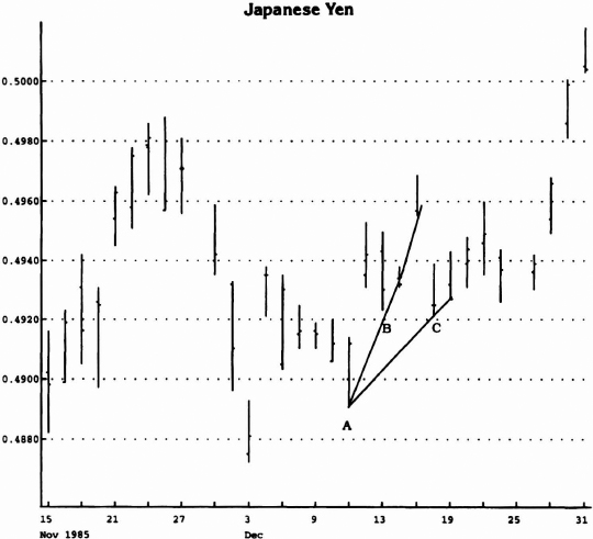
In Figures 1.4a,b, the two most recent peak descending TD Points™ were identified and then connected to construct the supply line (hereinafter referred to as a TD Supply Line™); in Figure 1.5, the two most recent ascending low pivot points were identified to construct the demand line (hereinafter referred to as a TD Demand Line™). It was that simple. No more excuses that I had selected the wrong points. The technique was now rigid and objective. Furthermore, the real attraction of this method of point selection was that it was dynamic. In other words, the market itself announced any changes in the supply–demand equilibrium equation by continuously resetting TD Points. Consequently, TD Lines are constantly being revised as more recent TD Points are being formed (see Figure 1.6). Once again, the importance of (1) the selection of the most recent TD Point and its connection to the second most recent TD Point as well as of (2) the construction of the TD Line itself becomes apparent.

Source: Logical Information Machines, Inc. (LIM), Chicago, IL.
Figure 1.4(b) Supply price pivot points (TD Supply Points) are resistance points that are defined by a high that is both preceded and succeeded, on the days immediately before and after, by lower highs. These TD Price Points are identified on the chart.

Source: Logical Information Machines, Inc. (LIM), Chicago, IL.
Figure 1.5 Demand price pivot points (TD Demand Points) are support points that are defined by a daily price low that is both preceded and succeeded, on the day immediately before and the day immediately after, by higher lows. The TD Price Points are identified on the chart.

Source: Logical Information Machines, Inc. (LIM), Chicago, IL.
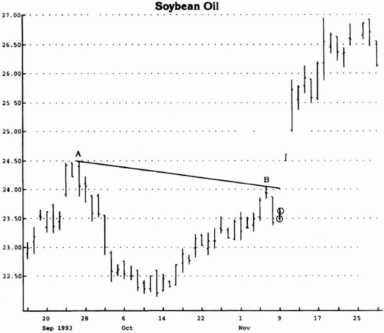
Figure 1.6 Four potential descending TD Supply Points are identified: A-B is the first supply line. Once TD Supply Point C is formed, however, a new supply line is constructed: B-C. Finally, when point D is defined, the supply line is revised to C-D. As you can see, the supply/demand balance is in a constant state of flux. Consequently, the supply line adapts to reflect these changes.
Refinements to TD Point Selection
I have found two modifications to the TD Point selection process to be helpful in some instances. Although they are not critical to your success in correctly selecting TD Points, they are presented for your consideration as well as for the sake of completeness.
An important factor when selecting TD Points relates to both the closes two days before the pivot high and the pivot low. In the case of the formation of a TD Point low:
- Not only must the lows the day before and the day after be greater than the lowest low—the low in between—but the pivot low must also be less than the close two days before the low.
In other words, should a price gap separate the low one day before the lowest low and the close the day before it, that close cannot be less than or equal to the lowest low (see Figure 1.7).
Source: Logical Information Machines, Inc. (LIM), Chicago, IL.
Figure 1.7 If the price gap defined as the distance from A to B—the price low (B) and the previous day's close (A)—is filled in, the low on the following day is no longer a demand point because the low is not less than the true low the previous day.
Conversely, in order to identify a TD Point high properly:
- 2. Not only must the highs the day before and the day after be less than the highest high—the high in between—but the pivot high must also be greater than the close two days before the high.
In other words, should a price gap separate the high one day before the highest high and the close the day before it, that close cannot be greater than or equal to the highest high (see Figure 1.8). As a matter of practice, some market timers differentiate between the highs and the lows that appear on a price chart and those that would appear if one were to fill in the price gaps. I coined the phrase for the former as “chart” highs and lows; and charting convention has labeled the latter as “true” highs and “true” lows.
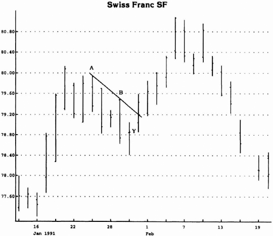
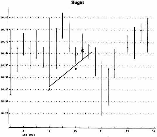
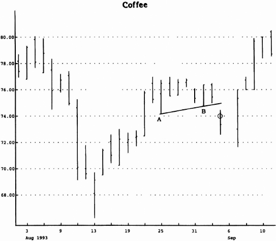
Having worked with TD Lines for a number of years, I was able to anticipate when the TD Points selected might prove invalid. My ability to subjectively validate these points was never defined or translated into decision rules until recently. By isolating the good examples from the bad, I was able to establish prerequisites that enabled me to perfect TD Point selection. This validation process involved the relationship between the most recent pivot point low or high and the close the day immediately following it. Specifically, if the close the day after the most recent pivot point low is below the calculated value of the TD Line rate of advance, the validity of that low is suspect (see Figure 1.9). Conversely, if the close the day after the most recent pivot day high is above the calculated TD Line rate of decline for that day, the legitimacy of that high is questionable as well (see Figure 1.10).
These refinements reduce the frequency of TD Points and, consequently, of TD Lines. At the same time, however, they serve to validate both the selection of the TD Points and the utility of the TD Lines in identifying support and resistance levels as well as in facilitating the process of calculating price projections.

Source: Logical Information Machines, Inc. (LIM), Chicago, IL.
Figure 1.8 Were the price gap between the high and the previous day's close considered, the supply point would not exist.
Benefits Derived from Proper TD Point and TD Line Selection
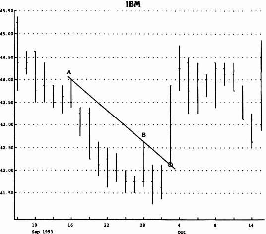
I was soon to learn that many benefits to this approach had been derived as a result of both the proper identification and the application of TD Points and of TD Lines. Inexplicable price gaps that had previously appeared out of the blue took on a special meaning and significance. Often, price vaulted above a TD Supply Line precisely at its intersection with price (see Figure 1.11). Conversely, this phenomenon was observed when price gapped below a TD Demand Line (see Figure 1.12). In addition, once price exceeded a TD Line, it became apparent that, in the ensuing price activity, a natural rhythm was dominant and was often predictable. For example, the extent of the price movement beneath a TD Line is often reflected in a comparable price movement above the TD Line (see Figure 1.13). Similarly, the degree of the price movement above a TD Line is often repeated beneath the TD Line (see Figure 1.14). The following discussion describes this technique in more detail.
Source: Logical Information Machines, Inc. (LIM), Chicago, IL.
Figure 1.9 In this instance, the close on the day immediately after the most recent pivot point low is below the rate of ascent as defined by the demand line connecting the two most recent ascending demand points. This occurs two times on the chart: lines A-B and A-C. Although it does not invalidate the demand lines, it raises questions regarding their reliability.

Source: Logical Information Machines, Inc. (LIM), Chicago, IL.
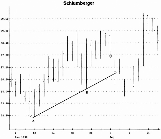
Figure 1.10 If the supply line constructed by connecting supply points A and B is extended, it intersects the day after supply point B, below that day's close. As you can see, a holiday gap appears on the chart and shifts price activity somewhat, but even if the chart is adjusted to accommodate this fact, the close one day after point B exceeds the line. Consequently, the value of that particular line is questionable.

Source: Logical Information Machines, Inc. (LIM), Chicago, IL.
Figure 1.11 See how price gapped upside above the TD Supply Line on the opening, and remained above all day.
Source: Logical Information Machines, Inc. (LIM), Chicago, IL.
Figure 1.12 Observe how price opened below the TD Demand Line.
Source: Logical Information Machines, Inc. (LIM), Chicago, IL.
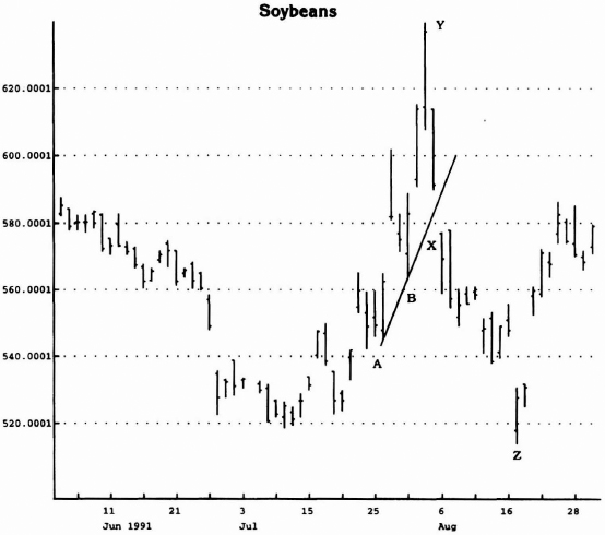
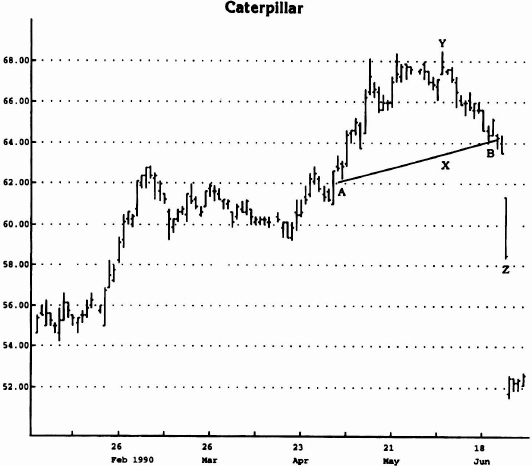
Figure 1.13 The price movement beneath the TD Supply Line A-B repeated only in reverse, once price exceeded the TD Line upside. The difference in price between the lowest price beneath the TD Line and the TD Line value on the same day is added to the breakout to arrive at a price objective. Specifically, price X on the TD Supply Line A-B is precisely above point Y, which is the lowest price recorded beneath the A-B Supply Line. By adding that value to the breakout above the A-B Supply Line, price projection Z is calculated.
Source: Logical Information Machines, Inc. (LIM), Chicago, IL.
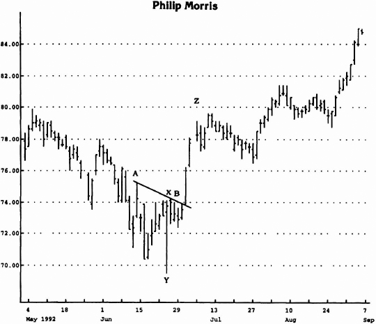
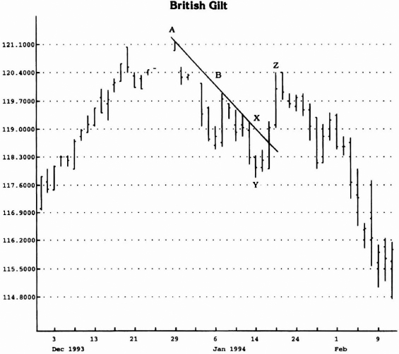
Figure 1.14 Price movement above TD Demand Line A-D is repeated in reverse on the downside, once the TD Line is penetrated. By calculating the difference between point Y—the highest price above the TD Line—and Point X—the specific price on the TD Line immediately beneath it—and by subtracting that value from the breakout below the A-B Demand Line, price projection Z is determined.
Price Projections
At the time I began to experiment with drawing trendlines on charts. I observed that if the price activity presented on the entire chart were bisected with a line separating, by an equal amount, extreme prices above and below that line, prices would often be drawn to and be repelled by that line (see Figure 1.15). I was fascinated. With a limited knowledge of trendlines, I continued to pursue the magnetic properties of this line. Having reviewed a considerable number of charts, I isolated as many common denominators as I could identify. You might say that this effort was both a precursor and a “back door” introduction to TD Lines. I mention this only to illustrate how I uncovered the unique property of symmetry in price movement.
Source: Logical Information Machines, Inc. (LIM), Chicago, IL.
Figure 1.15 The price activity is attracted to the line that bisects the price movement.
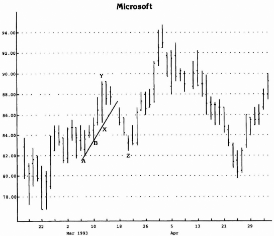
Earlier, I discussed the selection of TD Points and the construction of TD Lines. Once you are comfortable with the procedures required to perform these exercises, the phenomenon of price symmetry becomes apparent. Careful inspection reveals that the differences between extreme price points immediately above a TD Demand Line and the TD Demand Line itself, as well as immediately below a TD Supply Line and the TD Supply Line itself, replicate themselves once the TD Line is penetrated (see the discussion of TD Breakout Qualifiers in the last section of this chapter). Although the pattern itself is never precisely repeated, the extent of the movement both above and below the TD Line often is, and this behavior is what I describe as price symmetry.
TD Price Projectors
There are three distinct methods to calculate price projections once a trendline is penetrated validly; I call them TD Price Projectors. The particular technique selected is a function of the degree of precision and accuracy required by the user.
TD Price Projector 1, the least precise and the easiest to calculate, is as follows: when price advances above a declining TD Line, usually price continues to advance to at least a price level equivalent to the distance between the lowest price value beneath the TD Line and the TD Line value directly above it, added to the TD Line value on the day of the breakout to the upside. What may sound complex when described in words is very simple when viewed on the chart (see Figure 1.16).
Conversely, the identical symmetry is apparent when price declines below an ascending TD Line. Usually, price continues to decline to at least a price level equivalent to the distance from the highest price value above the TD Line to the TD Line value directly beneath it, subtracted from the TD value on the day of the breakout to the downside (see Figure 1.17). Often, visual inspection will allow the user to forecast approximate price objectives; most traders require more precision, however. Basic arithmetic will enable the user to calculate the rate of change of a TD Line simply by dividing the difference between the two TD Points by the number of days between them (excluding non-trading days). Further, by multiplying the additional number of trading days from the most recent TD Point to that precise point at which the TD Line is penetrated by the rate of change, the exact breakout value can be calculated (see Table 1.1). To that breakout value, the difference between the TD Line and the trough/peak immediately below/above—depending on whether it is a buy or a sell-can be added or subtracted to arrive at a price objective. Once again, what may appear complicated becomes much clearer when displayed on the charts (see Figures 1.18 and 1.19).
Source: Logical Information Machines, Inc. (LIM), Chicago, IL.
Figure 1.16 See how price gapped above A-B TD Supply Line and how by adding the difference between X—the value of the TD Line immediately above Y—and Y—the lowest price beneath the A-B Line—the price projection Z is determined.
TD Price Projector 2 is somewhat more complex. For example, in the case in which price exceeds a declining TD Line, instead of selecting the lowest price beneath the TD Line and adding that value to the breakout point, there is a slight variation. The intraday low price on the day of the lowest closing price beneath the TD Line is selected. Often, the lowest intraday low is recorded on the same day as the lowest close, so there exists no difference between TD Price Projectors 1 and 2; but, in those instances when the lowest close day and the lowest low day are not coincident, the adjustment is made.
Source: Logical Information Machines, Inc. (LIM), Chicago, IL.
Figure 1.17 In an uptrending market, TD Price Projector 1 concentrates on the extreme price high above the TD Demand Line. In this instance, price opened beneath A-B TD Demand Line and proceeded to satisfy price objective Z, which is calculated by subtracting the difference between the highest price above A-B Demand Line (Y) and the A-B value (X) on that same day from the price breakout.
Some examples will illustrate the distinctions between the two methods (see Figures 1.20 through 1.22). As you can readily see, using the intraday low as the reference point, regardless of the close that day relative to all other closes beneath the TD line, as TD Price Projector 1 requires, is considerably more liberal and simpler to calculate. On the other hand, TD Price Projector 2, using the intraday low of the lowest close day, is a little more difficult in arriving at a price objective once a declining TD Line is exceeded upside. Conversely, to arrive at downside price projections when an ascending TD Line is broken, the reverse procedure is employed (see Figures 1.23 and 1.24). In this case, the key day to concentrate on is the highest close day or, more precisely, the intraday high that particular day. Although it may appear that TD Price Projector 2 is more precise and conservative than Projector 1, this is not always the case. For example, if the rate of advance or decline is particularly steep and the lowest close in the case of a downtrend or the highest close in the case of an uptrend—the reference day for Projector 2—occurs before the intraday low or intraday high, then the price objective for Projector 2 is greater. Conversely, if the low or the high close day beneath or above the trendline occurs subsequent to recording the intraday low or high, then Projector 2 is less. Personally, I prefer Projector 1 to Projector 2, but I believe that Projector 2 is valid and is a viable option.
Table 1.1 Rate of Change Calculation of TD Line
|

Source: Logical Information Machines, Inc. (LIM), Chicago, IL.
Figure 1.18 In a declining market, TD Price Projector 1 concentrates on the extreme low price beneath the TD Supply Line. In order to arrive at a price objective Z, calculate the difference between X—the value on the A-B TD Supply Line—and Y—the lowest price recorded beneath A-B Supply Line prior to the price breakout—and add that value to the price breakout to arrive at the price objective. In strong markets, secondary price projections can also be made by multiplying the difference by 2.
Source: Logical Information Machines, Inc. (LIM), Chicago, IL.
Figure 1.19 Once the A-B TD Demand Line is constructed, TD Price Projector 1 requires that the price objective be calculated by subtracting value X—the price on the TD Demand Line on the day the peak price (Y) above the Demand Line is recorded—from Y and then subtracting the resulting value from the breakout to arrive at Z price objective.
Source: Logical Information Machines, Inc. (LIM), Chicago, IL.
Figure 1.20 Note, in this example, TD Price Projector 2 is the same as TD Price Projector 1 because the lowest close day (Y) recorded below TD Supply Line A-B is on the same day as the lowest low (Y).

Source: Logical Information Machines, Inc. (LIM), Chicago, IL.
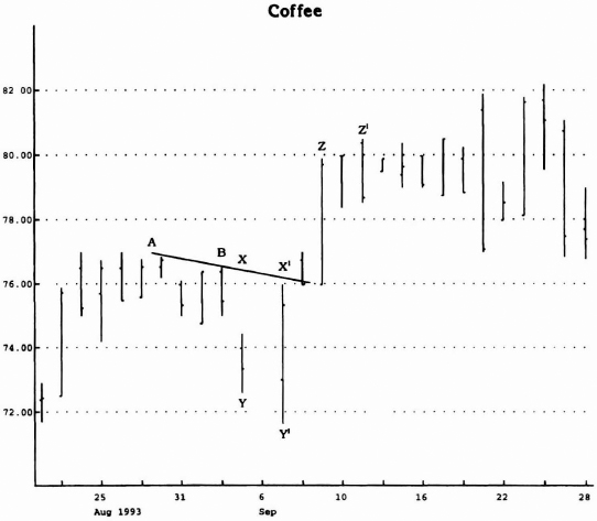
Figure 1.21 TD Price Projector 2 is not the same as TD Price Projector 1 in this example because the lowest close (Y) below TD Supply Line A-B is not on the same day as the lowest low (Y′). Even though the breakout point is the same value, the difference between Y and the value immediately above it on Supply Line A-B is different from the difference between Y′ and the value immediately above it on Supply Line A-B. Consequently, the price objectives are not the same.
Source: Logical Information Machines, Inc. (LIM), Chicago, IL.
Figure 1.22 The price objectives (Z and Z′), arrived at by subtracting the lowest low (Y′) beneath Supply Line A-B and the low on the lowest close (Y) beneath Supply Line A-B from the X and X′ values on the A-B line, are not the same in this case because the lowest close and the lowest low do not occur on the same day. Thus the distinction between TD Price Projectors 1 and 2.

Source: Logical Information Machines, Inc. (LIM), Chicago, IL.
Figure 1.23 TD Demand Line A-B defines two different downside price objectives (Z′ and Z) because the highest high day above the Demand Line (Y′) is not the same day as the highest close day (Y). This differentiates TD Price Projectors 1 and 2.

Source: Logical Information Machines, Inc. (LIM), Chicago, IL.
Figure 1.24 In both instances on the chart, lines A-B define the TD Demand Line, but the highest close above the TD Line (Y) and the highest intraday high above the TD Line (Y′) do not occur on the same day. Consequently, the price objectives for TD Price Projectors 1 and 2 are not the same.
TD Price Projector 3 is more conservative generally than the prior two methods. To calculate the price projection value in the instance of a declining TD Line, merely calculate the difference between the TD Line and the CLOSE of the lowest intraday low day immediately beneath it, NOT the intraday low itself (see Figures 1.25 through 1.27). The major distinction I wish to make relates to the intraday low and the close on the day of the intraday low. By definition, this approach is likely the most accurate in projecting prices because it usually yields the smallest returns. In order to reach the price targets established by TD Price Projector 1, the price objective generated by TD Price Projector 3 must have also been hit. Generally, this same observation applies to TD Price Projector 2, that is, the TD Price Projector 3 price target is realized first. Conversely, to project downside targets given a penetration of an ascending TD Line, the opposite procedure is conducted. The difference between the closing price of the highest intraday high day above the TD Line and the TD Line value immediately beneath it is calculated (see Figures 1.28 and 1.29). Once again, I emphasize the intraday high and the close on the day of the intraday high.

Source: Logical Information Machines, Inc. (LIM), Chicago, IL.
Figure 1.25 TD Price Projector 3 is conservative, and its price objective is generally realized prior to fulfillment of the price objectives for TD Price Projectors 1 and 2. This example demonstrates the selection of points for TD Price Projector 3. Note the close on the lowest day (Y) is near to the Supply Line A-B and, consequently, a lower target is generated once price breaks out above the TD Supply Line.
Source: Logical Information Machines, Inc. (LIM), Chicago, IL.
Figure 1.26 Once again, the upside price objective is muted because of the high close on the lowest low day relative to the Supply Line.
Of the three approaches presented to make price projections, TD Price Projector 3 is the most precise and the most conservative. Through experimentation, you should be able to select the approach with which you are most comfortable. I highly recommend that, regardless of which one you might select, you shave one price tick from the high, low, and TD Line when calculating the price projection, to compensate for rounding off and to ensure the likelihood of the price target's being realized. Specifically, when breaking an upsloping TD Line, subtract one tick from the high or the close, depending on the method used, and add one tick to the TD Line. Conversely, when breaking a downsloping TD Line, subtract one tick from the TD Line, and add one tick to the low or the close, depending on the method used.

Source: Logical Information Machines, Inc. (LIM), Chicago, IL.
Figure 1.27 This chart highlights numerous instances in which TD Price Projector 3 yields lower price targets than TD Price Projectors 1 and 2 because the close of the intraday low beneath the TD Supply Line (A-B) is used.
To fully comprehend the differences among the three TD Price Projectors, you should study Table 1.2, which summarizes the various similarities and differences.

Source: Logical Information Machines, Inc. (LIM), Chicago, IL.
Figure 1.28 Unfortunately, by using TD Price Projector 3, conservative price projections are made. As in this example, should the close on the lowest intraday low day beneath the TD Supply Line be positioned in the area of the high for the day, the price objective is less than if the close were positioned closer to the low for that day.
What Could Go Wrong?
No technique is perfect. Forecasting price movements, after all, cannot be that easy. What unexpected situations could arise? Three potential developments might occur, all of which can be dealt with simply:
- A contradictory signal could be generated by a penetration of an opposing TD Line. This would effectively nullify the active TD Line breakout and instate in its place, as the prevailing trend, the new TD Line breakout in the opposite direction. This is the most common way for a price trend to be terminated and for a price objective to be negated (see Figure 1.30).

Source: Logical Information Machines, Inc. (LIM), Chicago, IL.
Figure 1.29 TD Price Projector 3 requires that the difference between the close of the highest intraday high day above the A-B Line (Y) and the value of the A-B point (X) on that same day be subtracted from the downside breakout to arrive at the price objective.
- The initial indication of a valid TD Line breakout may be just plain false or may be reversed by an unexpected news event that dramatically shifts the supply–demand balance. This becomes immediately apparent when the open for the next day is recorded: and, on the opening, it either exceeds downside the value of the active descending TD Line, which was previously penetrated, and price continues to decline; or it gaps downside on the opening and, on the close, breaks below the descending TD Line. Conversely, the breakout is suspect when, on the next day, either the open or the close is recorded and either exceeds upside with a gap the value of the ascending TD Line it previously penetrated, and price continues to advance (see Figures 1.31 and 1.32). To reduce the financial risk associated with just such unforeseen events, a stop loss can be installed once price opens on the ensuing day.
Price Projector 1: Buy Signal—Calculate the difference between the lowest price low below the descending TD Line and the TD Line value immediately above it, and add that value to the breakout price. Sell Signal—Calculate the difference between the highest price high above the ascending TD Line and the TD Line value immediately below it, and subtract that value from the breakout price.
Price Projector 2:Buy Signal—Calculate the difference between the intraday price low on the day in which the lowest close below the descending TD Line is recorded and the TD Line value immediately above it, and add that value to the breakout price. Sell Signal—Calculate the difference between the intraday price high on the day in which the highest close above the ascending TD Line is recorded and the TD Line value immediately below it, and subtract that value from the breakout price.
Price Projector 3:Buy Signal—Calculate the difference between the close of the lowest intraday low below the descending TD Line and the TD Line value immediately above it, and add that value to the breakout price. Sell Signal—Calculate the difference between the close of the highest intraday high above the ascending TD Line ahd the TD Line value immediately below it, and subtract that value from the breakout price. 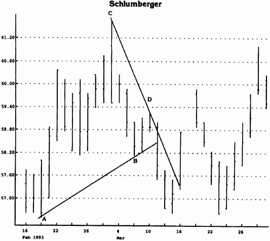
Source: Logical Information Machines, Inc. (LIM), Chicago, IL.
Figure 1.30 Note that the objective of Price Projector 1 had not been fulfilled for the breakout below TD Line A-B by the time an upside breakout of TD Supply Line C-D took place. Consequently, the downside price objective based on the penetration of the Demand Line A-B is no longer active.
- The fulfillment of a price objective defined by the breakout above or below a TD Line could disqualify an active trend. Such occurrences were discussed thoroughly earlier.
Source: Logical Information Machines, Inc. (LIM), Chicago, IL.
Figure 1.31 Although the TD Supply Line A-B was exceeded, on the day following the breakout the opening price was below the breakout day's close and it proceeded to immediately decline below the extended A-B Line. This price activity invalidates the breakout.
TD Lines of a Higher Magnitude
The TD Lines described and discussed above are of a level 1 magnitude, that is, each TD Point used to construct them required no more than three days to be defined—a high immediately preceded and succeeded by a lower high (or a low immediately preceded and succeeded by a higher low). The TD Line created by connecting two TD Points is of short duration, due to the fact that construction of as few as five highs (in the case of a TD Supply Line) or five lows (in the case of a TD Demand Line) could require two pivot points and immediately surrounding days. A trader may wish a longer-term perspective. To satisfy this requirement, I experimented with higher-level TD Points and Lines, and realized worthwhile results.
Source: Logical Information Machines, Inc. (LIM), Chicago, IL.
Figure 1.32 See how price failed to decline on the day following the penetration of the TD Demand Line A-B. In fact, price opened the following day unchanged and continued to advance from that price level above the extended A-B Line, thus nullifying the breakout.
To draw a TD Line of level 2 magnitude, a minimum of five days is required to identify each TD Point—a high immediately surrounded on both sides by two lower highs (or a low immediately surrounded on both sides by two higher lows). Similarly, a TD Line of level 3 magnitude would require a total of at least seven days for each, and so on for TD Lines of higher levels. It is correct to say that all TD Points of a magnitude greater than level 1 are also level 1 TD Points; but all do not qualify as active level 1 TD Line Points because, as discussed earlier, only the two most recent points are considered valid. To visualize this distinction, refer to Figures 1.33 and 1.34.

Source: Logical Information Machines, Inc. (LIM), Chicago, IL.
Figure 1.33 As you can see, level 3 magnitude TD Points are identified with a circle surrounding the high (low). [By definition, these are also level 1 magnitude TD Points as well. Those highs and lows marked with an “X” are level 1 points but do not qualify as level 3 because the highs (lows) all three days immediately before and immediately after are not lower highs (higher lows).]
Source: Logical Information Machines, Inc. (LIM), Chicago, IL.
Figure 1.34 The distinction between level 1 magnitude TD Points (“X”) and level 2 magnitude TD Points (circles) are apparent on this chart. Whereas level 1 requires merely a lower high (higher low) the days immediately before and after, level 2 requires two lower highs (higher lows) the two days immediately before and after.
Regardless which TD Line level of magnitude is selected, the same requirements exist as are described above for both TD level 1 Points and Lines. The only exception is the number of days required to define the TD Points. Similarly, the identical TD Price Projectors are used. It has generally been my preference, however, to follow level 1 magnitude TD Lines.
Source: Logical Information Machines, Inc. (LIM), Chicago, IL.
Figure 1.35 By awaiting the formation of a TD Point of a higher level of magnitude, lower-level TD Lines that are valid are forfeited. This chart illustrates two examples of valid breakouts that would have been identified had the points selected been level 1 or level 2 and not level 3 (see line A-B), and one example that would have been valid had level 1 been selected and not level 2 (see A′-B′).
I have two primary reasons for concentrating on the basic TD Line:
- As the level of magnitude increases, often the breakout occurs before the most recent TD Point is completely formed, and the trading opportunity is forfeited; consequently, the exercise becomes a game of “beat the clock” (see Figure 1.35).
Source: Logical Information Machines, Inc. (LIM), Chicago, IL.
Figure 1.36 TD Demand Line A-B (level 2) is active until price exceeds TD Supply Line A-B (level 2) upside. (Note how the breakout above the first TD Supply Line a-b correctly predicted the subsequent price movement and price objective.)
- As the level of magnitude increases, the likelihood of realizing the price objective before a contradictory signal occurs is reduced proportionately.
Occasionally, I will examine a higher-level TD Line to determine the trend defined by the TD Line and thereby to confirm that the TD Line I am using is consistent; in other words, I will refer to it to confirm my market outlook (see Figure 1.36).
Revolutionary Breakthrough: Validation of Intraday Price Breakouts
After the TD Points have been properly selected, the TD Line has been correctly drawn from right to left, the price objective has been calculated, and the three possible outcomes—(1) reversal signal, (2) dramatic shift in supply–demand equation, and (3) price fulfillment—have been addressed, there is one additional factor to consider: validation of intraday price breakouts. This element is significant. It is a major contribution to the study of market timing analysis. Furthermore, it has application to other techniques as well.
It's not surprising to hear that traders have taken positions on presumed trendline breakouts only to witness price fail and reverse and to incur significant losses. What is hard to understand, however, is that these same traders will continue to repeat this futile exercise and never question what causes it to occur. The incidence of false breakouts has always been high. They have been the nemesis of traders for years and have often been the excuse for totally abandoning the use of trendlines. The creation of TD Lines alleviates this problem somewhat, but invalid breakouts do occur occasionally. Heretofore, no method has been devised to differentiate between valid and invalid price breakouts.
Many years ago, I was involved in similar situations, became frustrated, and was determined to develop rules that would qualify TD Line breakouts. I was convinced that the TD Lines drawn were valid. I searched for a common denominator associated with both the good and the bad signals. It was not an easy task. The conclusions I made were startling and, at the same time, logical and simple. These were my findings.
I discovered three TD Breakout Qualifiers—two patterns occurring the day before a suspected breakout and the other pattern occurring the day of the breakout. Specifically, I concluded that if a particular market or index is oversold/overbought the day before a breakout, the chances are increased that the buying pressure/selling pressure would not be dissipated subsequent to the breakout, thus merely creating the illusion of continued strength/weakness.
Source: Logical Information Machines, Inc. (LIM), Chicago, IL.
Figure 1.37 Note that the closing price on the day immediately before the breakout to the upside was a down close versus the previous day's close. This pattern suggests an oversold condition prior to the breakout, which is a positive formation.
I experimented with numerous conditions precedent to a breakout and found that if the close the day before an upside breakout is down, the likelihood is increased that the intraday breakout will be valid and intraday entry is warranted—TD Breakout Qualifier 1 (see Figure 1.37). Further, if the close of the day prior to the upside breakout is up, the possibility of a false move exists (see Figure 1.38). Conversely, if the day before a downside breakout is up, the likelihood is increased that the intraday breakout is valid and intraday entry is warranted (see Figure 1.39). Further, if the close the day prior to the downside breakout is down, the likelihood of a false move exists (see Figure 1.40).
Source: Logical Information Machines, Inc. (LIM), Chicago, IL.
Figure 1.38 Observe that the close on the day prior to the upside breakout was an up close, thus indicating an overbought condition and the likelihood of a breakout failure.
An exception to the requirement that the close prior to an upside breakout be down and the close prior to a downside breakout be up was uncovered when an analysis of successful breakouts showed that not only would an oversold/overbought close qualify entry, but so would an open above a declining TD Line or an open below an ascending TD Line—TD Breakout Qualifier 2 (see Figures 1.41 and 1.42). This occurrence would suggest excessive strength/weakness and would justify entry at that opening price regardless of the previous day's close disqualifying the entry.
Source: Logical Information Machines, Inc. (LIM), Chicago, IL.
Figure 1.39 Note that the close on the day prior to the downside breakout was up, thus indicating a short-term overbought state and the likelihood of a valid breakout downside.
Source: Logical Information Machines, Inc. (LIM), Chicago, IL.
Figure 1.40 Notice that the close prior to the downside penetration of the A-B TD Demand Line was down, thus suggesting a false breakdown.
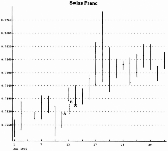
TD Qualifier 3 is similar to TD Qualifier 1 to the extent that it is based on price activity during the day prior to a breakout. In this case, however, the difference between the high and the close on the day prior to a trendline downside penetration is subtracted from that day's close to arrive at a supply value. The difference between the close and the low on the day prior to a trendline upside penetration is added to that day's close to arrive at a demand value (see Figures 1.43 and 1.44). If the ascending trendline is below the supply value and price exceeds the trendline, the price decline should accelerate and intraday action is warranted. Conversely, if the descending trendline is above the demand value and price exceeds the trendline, the price advance should accelerate and intraday action is warranted. Examples of TD Breakout Qualifier 3 are presented in Figures 1.45 and 1.46. Table 1.3 further describes the Qualifiers.
Source: Logical Information Machines, Inc. (LIM), Chicago, IL.
Figure 1.41 Observe that the opening price exceeded the TD Supply Line, thus validating a breakout.
As presented in this chapter, TD Points are objectively defined and, when properly connected, they create TD Lines. When TD Breakout Qualifiers are introduced and the TD Lines are penetrated, legitimate price breakouts are identified and price targets can be derived. It has never been so simple. Guesswork and lack of consistency are eliminated totally. Uniformity in construction, in application, and in interpretation has been accomplished. The successful identification of trends and of trend reversal points is complete.
Source: Logical Information Machines, Inc. (LIM), Chicago, IL.
Figure 1.42 See how price gapped on the open below the TD Demand Line, confirming a breakout.

Source: Logical Information Machines, Inc. (LIM), Chicago, IL.
Figure 1.43 By calculating the difference between the close on the day prior to an upside breakout and that same day's low (or the previous day's close, whichever is less) and adding that difference to the close prior to the breakout, validation of the breakout is determined. If the difference added to the close is less than the breakout price, a valid breakout is identified. If the difference is greater than the breakout price, a false breakout is likely to occur. Specifically, in this example, the difference between the close and the low on the day prior to the breakout above TD Supply Line A-B is calculated and it is less, thus qualifying the breakout. TD Demand Line A′-B′ is also drawn, and the same concept in reverse qualifies the downside breakout (see Figure 1.45).
Source: Logical Information Machines, Inc. (LIM), Chicago, IL.
Figure 1.44 The difference between the close and the low on the day prior to the upside breakout of A-B Supply Line added to the close on the day prior to the breakout is less than the breakout price. Consequently, a valid breakout has been confirmed.

Source: Logical Information Machines, Inc. (LIM), Chicago, IL.
Figure 1.45 By subtracting the difference between the high one day before a downside breakout (or the close two days before it, if it is greater than the high one day before the breakout) and the close the day before the breakout from the close that same day, the breakout can be validated. In this instance, the A-B Demand Line was less and the breakout was validated.

Source: Logical Information Machines, Inc. (LIM), Chicago, IL.
Figure 1.46 The difference between the close and the low the day before the breakout added to the breakout is less than the breakout price, thus validating the breakout.
Table 1.3 TD Breakout Qualifiers
| TD Breakout Qualifier 1: |
| To validate a buy signal, the close the day before a buy signal is a down close. |
| To validate a sell signal, the close the day before a sell signal is an up close. |
| TD Breakout Qualifier 2: |
| To validate a buy signal, a price open greater than the breakout price must occur. To validate a sell signal, a price open less than the breakout price must occur. |
| TD Breakout Qualifier 3: |
| To validate a buy signal, the value arrived at by adding the difference between the close and the low the day prior to a breakout or the close 2 days before whichever is less to that same day's close must be less than the breakout price. To validate a sell signal, the value arrived at by subtracting the difference between the high or the close 2 days before whichever is greater and the close the day prior to a breakout from that same day's close must be greater than the breakout price. |