
Chapter 2
Retracements
Price advances and declines do not continue uninterrupted. Contratrend rallies and trend reversals occur all the time. Predicting the extent and the duration of these moves is a preoccupation of market analysts. Techniques to project these retracement levels, however, are not only inexact but also often haphazardly applied. Generally, little preparation and forethought are given to the selection of the points critical to the calculation of both support and resistance levels. Through trial and error, I have identified proper price selection techniques, as well as ratios, that can be universally applied to all markets. I have replaced the practice of random selection and guesswork with an objective, mechanical approach that offers a series of explanations and includes examples to justify my techniques.
Selection of Points and Retracement Ratios
In the summer of 1973, one of my senior business associates gave a compelling speech forecasting a steep retracement rally for the stock market to be completed by early fall. When quizzed regarding the upside potential, he flatly stated that he expected an advance approximating three-eighths to five-eighths of the previous decline. When asked to be more precise, he was unable to do so. When asked how he arrived at these figures, he flippantly responded that most rallies in a bear market expire at one of these two levels. He could not supply any additional information other than the fact that he had read of similar ratios in a market letter and suggested I contact the writer to learn of the significance and origin of these numbers. When I called, the writer made reference to a market analyst by the name of R. N. Elliott and an article he had written in Financial World many years earlier. At the library, I was able to retrieve the article from the archives. What I read regarding Fibonacci numbers was fascinating and informative. Unfortunately, it proved to be woefully incomplete. I began an exhaustive examination of price activity to uncover a precise, objective approach to calculating retracements. My goal was to identify a method that was mechanical and had application to all markets. The conclusions of my research are presented in the following discussion.
Rather than devote a lengthy amount of time and space to a discussion of Fibonacci numbers and their presence and dominance in nature and in surroundings, I recommend, should you desire further information, that you consult the numerous recent textbooks and articles dealing with the subject matter and the “golden mean.” Briefly, I highlight the significance of the Fibonacci time series starting with the numbers 1, 2, 3, 5, 8, 13, 21, 34, 55, … and so on. Essentially, these numbers are obtained by summing two consecutive numbers in the series to arrive at the next number. As the numbers increase in size, the ratio obtained by dividing a preceding number by a succeeding number approaches .618, and, conversely, the ratio obtained by dividing a succeeding number by a preceding number is 1.618. This is a characteristic peculiar only to this specific time series.
I apply these numbers and ratios to much of my work. Specifically, in the case of retracements, I use what has become the standard, the “mother of all retracement ratios”: .618. I believe that in the early 1970s I was the first to apply .382 (1.00 – .618) retracements as well. The retracements increase from .382 and .618 to unity or “magnet price” (not 1.00, as most believe, but the high/low day's close, depending on whether the correction is up or down). From the full retracement to the magnet price, they continue 1.382, 1.618, and 2.236 (1.618 + .618), and in the case of a market recording all-time, record highs, the actual ratios .618 and .382 times the absolute price high. The series of retracement levels are described below (see Table 2.1).
More important than the ratios themselves is the selection of the price points required to calculate the retracements. For most analysts, such a process is a moving target. Once again, in order to maintain consistency and uniformity, I refined and defined these price levels precisely and objectively. My research suggested that the best results were obtained by applying the following procedures.
Assume a recent low has been recorded. To establish reference points for retracement price objectives, extend an imaginary horizontal line from that recent low toward the left side of the chart to the last time a lower low had been recorded (see Figure 2.1). Next, refer to the highest price between these two points; that is the “critical price.” By subtracting the recent low from that value, price retracement levels can be projected (see Figure 2.1). Conversely, to arrive at retracement levels off a price peak, the same exercise is performed in reverse. Specifically, extend an imaginary line from the recent price high toward the left side of the chart to the last time a higher high was made (see Figure 2.2). Identify the lowest low between these two points; that is the critical price. By subtracting the critical price from the recent high, price retracement levels can be projected (see Figure 2.2). Not only is this approach simple but it ensures that the calculation of retracements will always be clear, well-defined, and uniform.
| .382 |
| .618 |
| Magnet price (high/low day's close) |
| 1.382 |
| 1.618 |
| 2.236 |
| 2.618 |
| 3.618 |
Source: Logical Information Machines, Inc. (LIM), Chicago, IL.
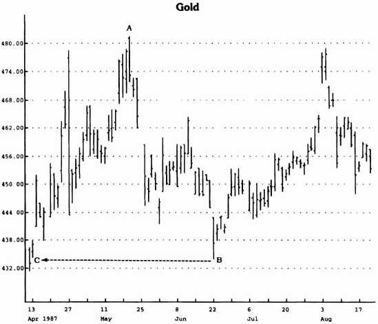
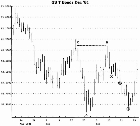
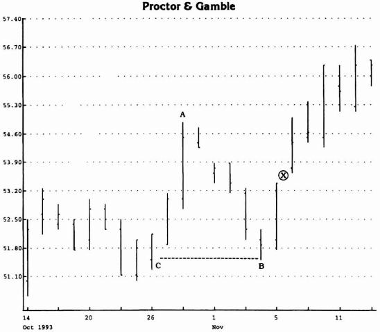
Figure 2.1 Once price level B has been defined, refer, on the left side of the chart, to the last time a lower low than that registered on day B was recorded (see price C). The highest high between these two points (A) is the critical price and is an important reference level when calculating upside retracements. By calculating the price difference between points A and B and multiplying by retracement factors, upside projections can be made. Notice how price hit an important obstacle at point A's close and not at the intraday high (refer to the discussion regarding magnet price and to Figure 2.5).
Source: Logical Information Machines, Inc. (LIM), Chicago, IL.
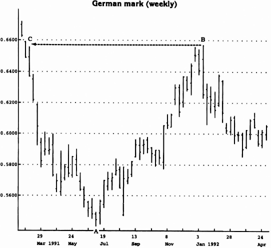
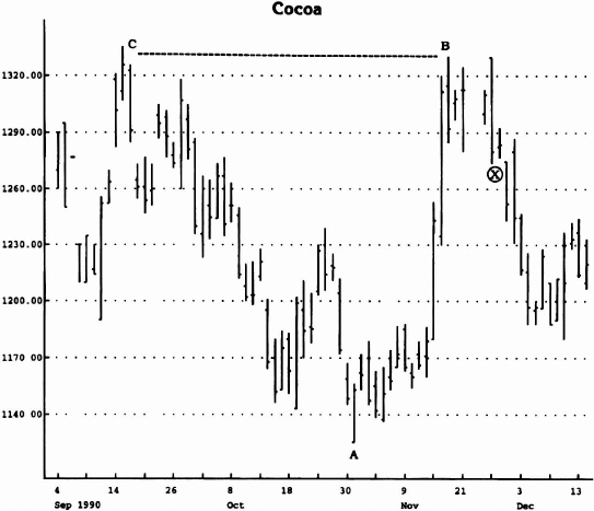
Figure 2.2 To calculate the downside retracement levels, extend an imaginary line toward the left side of the chart to the last time a price high exceeded the high of point B (see price C). The lowest low between these two points (A) is the critical price and a key level when calculating downside retracements. By calculating the price difference between points A and B and multiplying by retracement factors, downside price projections can be made.
Experience has proven that the initial retracement levels of .382 and .618 are valid and predictable when the critical price point is properly identified (see Figures 2.3 and 2.4). However, most analysts who had even accidentally selected the correct points were mistaken when they assumed that, once price had exceeded both the .382 and .618 levels, the next objective was the critical price day's high in the case of a rally and the critical price day's low in the case of a decline. In actuality, this widespread expectation has served for years as merely a decoy for unsuspecting traders (see Figure 2.5). My research with retracements many years ago uncovered a more crucial level, which served as a resistance/support level. Consequently, I refer to this price as the “magnet price.” How often have you awaited penetration of a critical price high/low to liquidate or to enter a trade, only to witness price reverse direction early without a fill? In other instances, it is not uncommon to see price accelerate through a critical price and immediately proceed to the 1.382 level, just at the time when everyone expects support at the intraday low or resistance at the intraday high. Unexpected movements occur at this price level when one is not properly prepared.
Source: Logical Information Machines, Inc. (LIM), Chicago, IL.
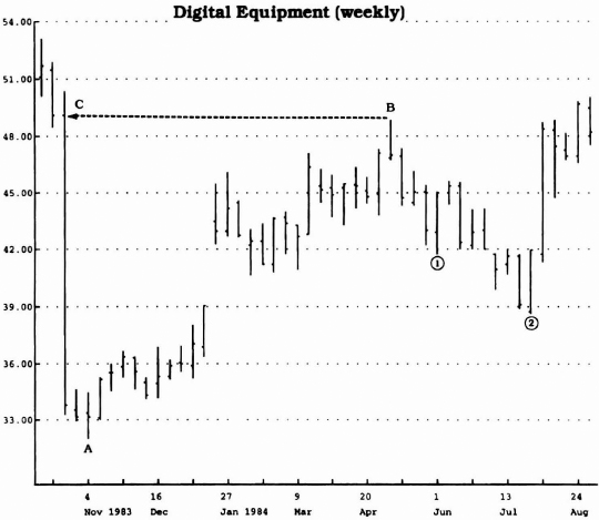
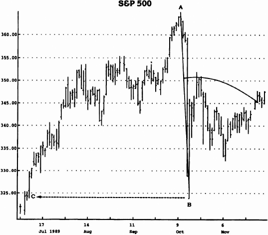
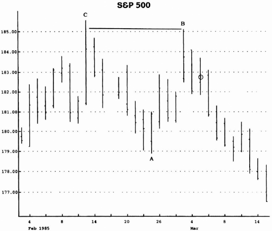
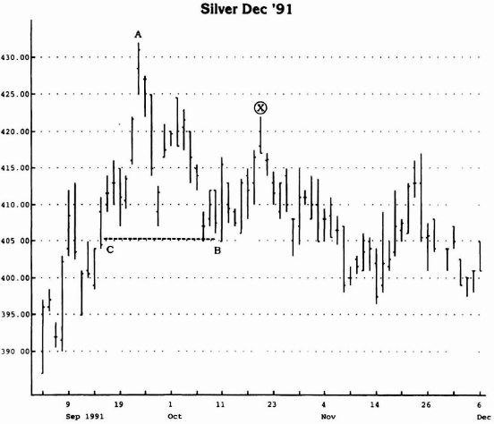
Figure 2.3 By identifying the lowest low between points B and C—the recent high (B) and the last time a higher high was recorded (C)—downside retracement levels can be calculated. Marked on the chart are levels 1 and 2, which identify .382 and .618 retracements of the move from point A to point B.
Source: Logical Information Machines, Inc. (LIM), Chicago, IL.
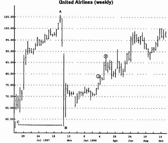
Figure 2.4 By identifying the highest high between points B and C—the recent low (B) and the last time a lower low was recorded (C)—upside retracement levels can be calculated. Marked on the chart are levels 1 and 2, which correspond with .382 and .618 retracement levels of the move from point A to point B.
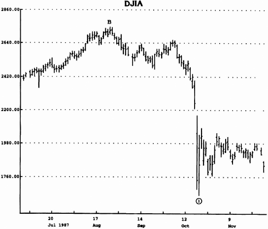
There are exceptions to the retracement calculations presented above. Experience suggests that the previous examples are associated with trading range markets. Once price advances to record all-time highs, however, the selection of a “critical point” (low) is impossible, because no other high exists farther left on the chart. In these instances, I have found multiplying the absolute peak price by .618 and by .382 works well. Two instances are indelibly etched upon my memory. The first is a forecast I made to an audience in New York prior to the 1987 stock market crash. At that time, the August price high for the Dow Jones Industrial Average was approximately 2747—a record. By multiplying that value by .618, I was able to calculate a support (retracement) level for the market of approximately 1697 (see Figure 2.6a). I presented that level to the audience as my downside price projection. At the same time, I presented a TD Line breakout objective of 1650 (see the trendline discussion in Chapter 1). Although mechanically and objectively derived in both instances, it was surprising how both reinforced one another and lent credibility and conviction to my forecast.
Source: Logical Information Machines, Inc. (LIM), Chicago, IL.
Figure 2.5 Observe how price retraced to levels 1 and 2 and eventually declined to the low day's range exceeding that day's close. How many traders were expecting a test of the low price at point A and were fooled? The key is the “magnet price”—low day's close.
Source: Logical Information Machines, Inc. (LIM), Chicago, IL.
Figure 2.6(a) If one were to extend an imaginary line from point B to the last time price recorded a higher high to identify a reference low in between, he would be unable, because price had never been higher. In these rare instances, valid downside price projections can be calculated by merely multiplying the absolute high by .618 and by .382. In this example, price met good support at level 1, which approximates .618 times the high.
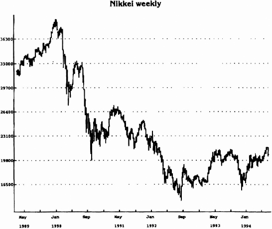
Another episode involving the application of this retracement approach relates to a forecast I made subsequent to the Nikkei Average recording its all-time high at 38957. I had been sponsored by a large brokerage house and was invited to make a series of speeches in Japan regarding various Japanese markets. Invariably, the topic would be directed to the Japanese stock market. Due to the fact that a record high had been realized and that no “critical price” (low) could be identified, I applied my approach to the Nikkei Average. As you can see on Figure 2.6b, the technique accurately predicted the downside price objective below 15,000. At the time the forecast was made, skepticism and ridicule were common. Once price had accomplished this downside objective, however, respect for the technique was pervasive.
Source: Logical Information Machines, Inc. (LIM), Chicago, IL.
Figure 2.6(b) Using the DeMark technique to predict the downside price objective.
TD Retracement Arcs
Another method I developed many years ago projects retracement levels incorporating both price and time. I had never seen anything quite like it prior to my research and have never seen anything similar since. Instead of identifying one retracement price objective as most other techniques do, this approach has a floating price objective that adjusts to the passage of time. More specifically, the price objective changes from day to day. The specific price resides on an arc.
Source: Logical Information Machines, Inc. (LIM), Chicago, IL.
Figure 2.7 This unique approach incorporates both price and time. The reference points are identified the same as before, but once identified the two points are connected with a straight-edge ruler and the retracement levels (.382, .618, and the magnet price) are identified on this line. Then, by using point B as a fulcrum, an arc is extended to the right of the chart; once a price close exceeds the arc in the future, it proceeds to the next TD Retracement Arc level. This assumes that the points are properly anchored to avoid any changes in the shape in the arc when either the price or the calendar scale is changed.
The arc is constructed by drawing a line that connects the critical price and the recent low/high, depending on whether an advance or a decline is expected. Once the .382 and the .618 points on the line itself are identified, the recent low/high serves as a fulcrum or a pivot point for an arc that extends from those points into the future. The curve that appears describes retracement projections (see Figures 2.7 and 2.8). As price declines below/above the pivot point, a new arc must be drawn.
Source: Logical Information Machines, Inc. (LIM), Chicago, IL.
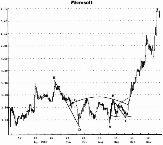
Figure 2.8 Note the numerous TD Retracement Arcs formed by lines extending from points B-A, C-B, and D-E. The arc formed by B-A is reversed by the arc defined by C-B, and the price breakout upside above the latter arc is confirmed by a similar breakout above the larger TD Retracement Arc D-E.
Retracement Qualifiers
Important elements of my TD Lines are the TD Breakout Qualifiers (see the discussion of TD Line in Chapter 1). They are extraordinary filters that predetermine whether an intraday breakout is valid or invalid. So too, moves exceeding .382 and .618 retracements can be prescreened as legitimate or not. My research suggests that these same TD Breakout Qualifiers apply equally well to validating retracements. To remain consistent with the topic, however, I refer to these qualifiers as TD Retracement Qualifiers 1, 2, and 3. It might be worthwhile to reiterate their respective definitions. Specifically, TD Retracement Qualifier 1 requires that the close on the day prior to an advance above the retracement level be down in order to qualify for intraday entry and the expectation that the advance will continue (see Figure 2.9). Conversely, it provides that the close on the day before a decline below the retracement level be up in order to qualify for intraday entry and the expectation that the decline will continue (see Figure 2.10). Should this qualifier in either situation be lacking, the potential of the advance or the decline reversing, rather than accelerating, at those precise points increases significantly. Another possibility exists, and that is TD Retracement Qualifier 2. In this instance, both an upside and a downside penetration can qualify, provided price exceeds the retracement level on the opening (see Figures 2.11 and 2.12). This occurrence suggests that the price dynamics are so strong that entry is validated and that the continuation of the move is imminent. One additional qualifier (TD Qualifier 3) can be incorporated into one's trading arsenal. The concept of overbought/oversold is employed in this instance just as with TD Qualifier 1, but the approach is different. Specifically, the expression of supply or demand is calculated on the day prior to the breakout. The difference between the previous day's high and that day's close is subtracted from that day's close to arrive at a supply value; conversely, the difference between the close and the low on the day prior to the breakout is added to that day's close to determine a demand value (see Figures 2.13 and 2.14). Just as when the TD Line on a particular day is below the supply value or above the demand value and a legitimate breakout is recorded by price exceeding the TD Line, so too the same approach applies to retracement points. In fact, in those exceptional instances when both the TD Line and the retracement levels are qualified, they appear to reinforce one another and translate into successful trades.
Source: Logical Information Machines, Inc. (LIM), Chicago, IL.
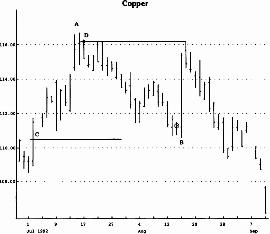
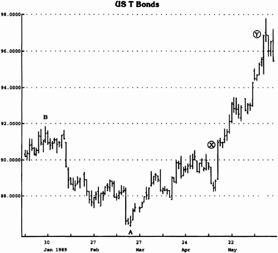
Figure 2.9 The close on the day before point B is a down close (circled), which satisfies TD Retracement Qualifier 1, indicates an oversold condition, and improves the prospects for intraday entry and a successful trade to the retracement levels. In this instance, the .382 and the .618 retracement levels were fulfilled the same day. In fact, the move the following day extended to the magnet price (D)—point A close—and did not, as most traders would expect, reach point A day's high.
Source: Logical Information Machines, Inc. (LIM), Chicago, IL.
Figure 2.10 The close the day before the .618 retracement level was an up close (circled) and implied a valid retracement, as well as justified intraday entry. TD Retracement Qualifier 1 has been satisfied.
Source: Logical Information Machines, Inc. (LIM), Chicago, IL.
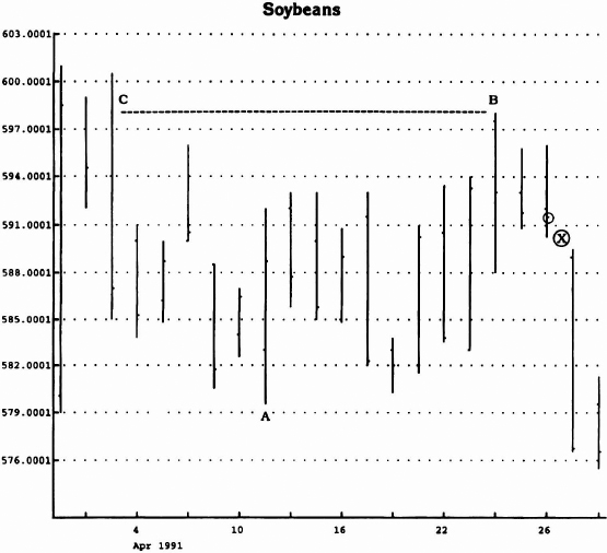
Figure 2.11 See the opening gap downside (X) below the .382 retracement level. This fulfills the requirement of TD Retracement Qualifier 2 and negates the fact that the previous day's close was a down close (see circled close).
Source: Logical Information Machines, Inc. (LIM), Chicago, IL.
Figure 2.12 Price gapped above the .618 retracement level and fulfilled Retracement Qualifier 2 in the process.
Source: Logical Information Machines, Inc. (LIM), Chicago, IL.
Figure 2.13 By calculating the difference between the high the day before penetration of a retracement level (or the close the previous day, whichever is greater) and the close the day before the breakout, and subtracting that value from that close and then comparing it with the retracement level, it can be determined whether price will continue to the next lower retracement level or reverse. If the retracement price is below the value, then price should continue to decline; if the retracement price is above that value, then price should attempt to rally. The difference between the high and the close the day before X retracement level is above the .382 retracement point; consequently, price continued to decline. TD Qualifier 3 has been fulfilled.
As displayed in Table 2.1, there exists a series of retracement levels; when one is exceeded, price gravitates typically toward the next level. Not included in Table 2.1 nor in the earlier discussion, however, is a hybrid situation that refines retracement expectations even further. Despite the fact that price may exceed a retracement level and that a retracement qualifier may have been satisfied, a situation may arise in which the closing price is unable to remain in excess of the retracement value. Provided that the closing price does not fail to exceed the previous day's close, the only adjustment required is a minor one. Instead of the next retracement level being the one listed in Table 2.1, it is actually one-half of the distance between the two levels. For example, if price exceeds the .382 retracement level, is properly qualified, and closes above the previous day's close but fails to close above the .382 retracement level, the expectation level is no longer a .618 retracement objective; rather it is the 50 percent level. Furthermore, should all prerequisites be satisfied at the .618 level but the closing price fail, the revised retracement level would be one-half the distance from .618 to the critical price or the magnet price, whichever is less. The same process occurs, in reverse, when price declines.
Source: Logical Information Machines, Inc. (LIM), Chicago, IL.
Figure 2.14 Price failed at the retracement level because the difference between the previous day's close and low added to that same day's close was greater than the retracement level.
A final variation of retracements incorporates both price and time, as does the TD Retracement Arc. Rather than identify on an arc the time and the price retracement level, this approach applies a meter to the amount of time allotted to accomplish penetration of the retracement level. For example, if the number of days from a peak to a low is counted and this value is multiplied by .382, an expiration time in which to fulfill a retracement is defined. The same concept can be applied to larger retracements, such as .618.
During the mid-1970s, in order to simplify the process of calculating price retracements, I purchased a proportional divider. I ordered this device from Teledyne-Post and it had to be sent from overseas. Since that time, I have shared this tool with many other market analysts and subsequently they have purchased their own. I recommend that if you work with price charts and if you quickly want to approximate retracement levels, then purchase one from your local art or drafting supply store.
The discussion above describes methods to objectively define the parameters for calculating and qualifying retracements. The beauty of these approaches is that they are totally objective. No allowance for subjective interference or for personal bias is permitted. In the final analysis, no excuses can be attributed to faulty suppositions. Everything considered is hard and fast, with clearly defined rules for application and interpretation.
Trend Factors™
Often, both traders and investors preoccupy themselves with market rhetoric. As far as I am concerned, however, one distinction they fail to recognize or to acknowledge is the difference between the duration and the degree of price moves. Invariably, were I to ask for definitions to widely used market terms such as short, intermediate, and long term, I would wager that most, if not all, would respond in temporal terms. Although the responses might vary somewhat, I would expect to hear that short term relates to moves of less than one month's duration, intermediate term to moves longer than one month but shorter than six months, and long term to moves lasting more than six months. These labels may have been appropriate prior to the 1980s, but because of increased volatility in the financial markets, they have become outdated. Moves that in the past consumed weeks or months are being fulfilled in days or hours. Because of market illiquidity, the speed of news dissemination, the herd instinct of fund managers, and other factors, this trend continues. Consequently, I apply the descriptions of short, intermediate, and long term to percentage price movements rather than to specific time intervals. For example, I consider moves of less than 5 percent to be short term, moves of 5 to 15 percent to be intermediate term, and moves greater than 15 percent to be long term. These definitions apply regardless of the time required to accomplish these moves. In this context, I rely on an analytical tool I developed many years ago to forecast the inception of trend moves of an intermediate to long-term variety. I refer to the set of specific ratios I use as Trend Factors™.
In the early 1970s, I observed a dominant tendency for various markets to exhibit support and resistance at price intervals defined by percentage retracements from preceding price peaks and troughs. For example, upside resistance levels were projected by multiplying a recent low by a series of prescribed ratios. Conversely, downside support levels were calculated by multiplying a recent price peak by the inverse of the upside ratios. Through a tedious trial-and-error process. I was able to approximate the ideal ratio values. I established prerequisites to qualify the reference highs and lows and to ensure consistency and uniformity. The selection criteria necessary to identify the correct reference value—whether high, low, or close—were critical to defining the price trend and the anticipated price movement.
In order to define it, a reference low must first be qualified. Because the minimum Trend Factor ratio is .0556, a qualified low exists once price has declined to a value at most .9444 from a previous qualified reference high day's close (see Figure 2.15). Conversely, a qualified high exists once price has advanced the minimum Trend Factor 1.0556 from a previous qualified reference low day's close (see Figure 2.16). It's that simple to select price points that qualify. Before getting too specific, I'd like to introduce you to the concept of Trend Factors™.
Source: Logical Information Machines, Inc. (LIM), Chicago, IL.
Figure 2.15 From point B to point A, price declined more than .0556—in other words, the value of point A is no more than .9444 times the value of point A. This validates point A as a Trend Factor low. Price X is the 1.0556 level and price Y is the 1.112 level.
Source: Logical Information Machines, Inc. (LIM), Chicago, IL.
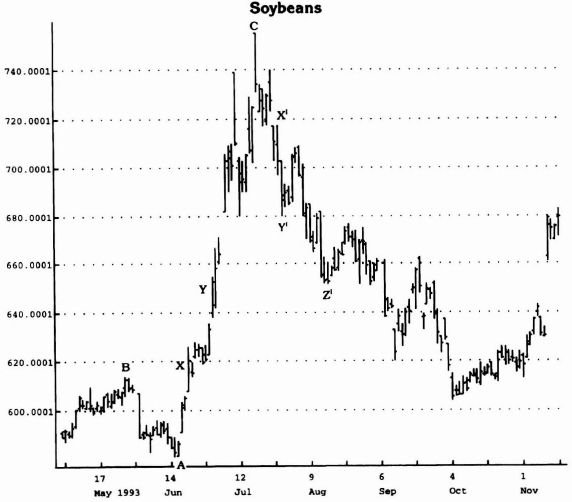
Figure 2.16 Point A is no more than .9444 point B and is qualified as a reference point. Price levels X and Y correspond to 1.0556 and 1.112 Trend Factor objectives. Point C qualifies as a Trend Factor high reference point because price advanced from point A by more than 1.0556. X′ and Y′ identify Trend Factor objectives, as does Z.
There appears to be a critical juncture in price movement, at which point, once price momentum surpasses on a closing basis key support or resistance levels, it is able to proceed to the next critical juncture. The market itself legitimizes those price moves. An alert trader can capitalize on the message the price movement sends once it exceeds these critical price levels. Figures 2.15 and 2.16 demonstrate this phenomenon. As identified earlier, the essential ingredients are the qualification and the selection of the reference point and then the Trend Factor ratios. To determine the first level of resistance upside, the reference point must be multiplied by 1.0056: to arrive at the second level of resistance upside, the reference point must be multiplied by 1.112 (2 × .0556); and to calculate the third level of resistance, the reference point must be multiplied by 1.14 (2½ × .0556). On the other hand, to determine the first level of support downside, the reference point must be multiplied by .9444; to arrive at the second level of support downside, the first downside target must be multiplied by .9444 again (this is different from the upside process); and to calculate the third level of support downside, the second level must be multiplied by .9722 (½ of value between .9444 and 1.000).
It is important to select the proper reference price value, to ensure that the support and the resistance levels are defined accurately. My research has confirmed that specific patterns identify what price to use to calculate these threshold levels. Specifically, if (1) the reference day's close is less than the close one day earlier, and (2) the close one day before the reference day's close is less than the close two days earlier, and (3) the close one day after the reference day's low is greater than the reference day's close, then the upside resistance level and projection values are determined by multiplying the reference day's low by the ratios. If either the reference day's close or the close one day before is an up close or an unchanged close, then the reference price used to calculate the first resistance level is the reference day's close. The only exception arises when the low the day after the reference day exceeds the close of the reference day. In this instance, the first level of resistance is determined by multiplying the close on that day by the ratio 1.0556 (see Figure 2.17). The second and third levels of resistance are calculated by using the reference day's low.
When defining the first level of support, as well as the next two levels of downside price projections, a similar evaluation of closing price relationships must be done. If the close of the reference day as well as the day prior to the reference day are up closes, then the high of the reference day is used to project the critical support level and the second support level is projected by multiplying the first support level by .9444. The third support level is .9722 times the second. If either the close the day before the reference day or the close the day of the reference day is a down close, then the same ratio is multiplied by the reference day's close. The only exception arises when the high the day after the reference day is less than the reference day's close. In this instance, the first level of support is determined by multiplying the close that day by the factor .9444 (see Figure 2.18). The second and third levels of support are calculated by using the reference day's high.
Source: Logical Information Machines, Inc. (LIM), Chicago, IL.
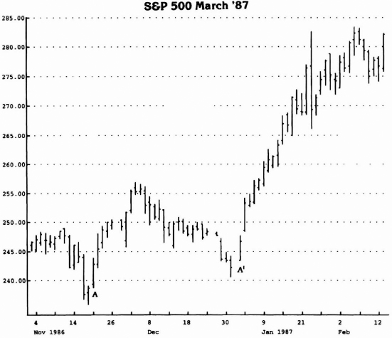
Figure 2.17 A and A′ identify days after reference lows in which price gaps exist—the low fails to intersect the previous day's close. Consequently, the Trend Factors are multiplied by the closes on these days.
Source: Logical Information Machines, Inc. (LIM), Chicago, IL.
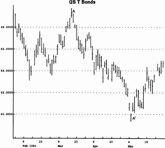
Figure 2.18 A identifies a day on which the high does not intersect the previous day's close and, consequently, a price gap exists. The Trend Factor is multiplied by the close on that specific day. A′ identifies a reference low defined by an upside gap.
Generally, the first attempt to exceed level one, established by the low or the high multiplied by the Trend Factor, is accomplished easily. However, in those instances where price exceeds the projection and closes in the direction of the trend but fails to close above or below it, the next trend factor objective is reduced by 50 percent—specifically, level two price projection is 1.0834 and .9722. These exceptions apply only when price confirms level one intraday but not on a close.
One exception to those rules does exist. Due to the fact that some futures' markets are quoted in decimals such as the currencies, and are not preceded by any whole numbers, it is important to adjust the Trend Factor™, to include another prefix—.99444 instead of .9444 and 1.00556 instead of 1.0556.
I have found that the support and the resistance levels projected by utilizing Trend Factors™ are often uncannily exact (see Figure 2.18). It is not uncommon to witness price approach a level or even exceed it intraday, only to then fail and reverse trend at precisely the Trend Factor™ level. Conversely, once a defined level is exceeded on a closing basis, price generally proceeds to the next level. The keys to success when using this approach revolve around the selection of reference points and the proper implementation of the Trend Factors™. The same filters discussed earlier in this chapter can be applied equally well to qualify anticipated breakouts.