
Chapter 5
Accumulation/Distribution
My introduction to conventional technical analysis and to its preoccupation with subjective and artistic interpretations left me totally frustrated. Consequently, I rebelled and reverted to the other extreme: I searched for techniques that were totally objective and mechanical. At the same time I was poring over charts and divining mechanical chart techniques, I employed my economics and mathematics background to create supply–demand models capable of identifying buy and sell opportunities. My journey to accomplish this goal is described in this chapter.
Although I initially experimented and developed these various techniques for the equity markets, my research confirmed that, with a few minor adjustments, these same methods could be applied to the futures markets. Through the use of various price volume studies and formulas, I ultimately created the product that satisfied my needs.
I had learned in Economics 101 that an increase in demand occurring at the same time as static or diminishing supply translated into an advance in price. Conversely, an increase in supply that was coincident with constant or reduced demand caused price to decline.
With those principles in mind, I researched all the techniques I could find that dealt with price movement and volume. This mission included the basic on-balance volume approaches used by various market analysts. Specifically, in these instances, price activity was compared to numerous volume-weighted calculations. The basis for this type of analysis was simple: volume is considered the fuel required to move prices up and down. By successfully identifying whether the big buyers are accumulating or distributing their positions, a trader can benefit by them. Big-block stock activity is generally associated with large, sophisticated, and informed investors. To capitalize on and to participate in both their research and expectations, it is important that a market model be sensitive to shifts in supply and demand caused by their campaigns.
I have always described technicians as parasites because, in the truest sense, they are not informed nor do they care about the fundamental factors contributing to investment decisions. Their only goal is to identify and to ride the trend. An episode that occurred many years ago demonstrates the truth of this statement and best typifies the personality and attitude of a pure trader. I introduced a close friend of mine to one of the market timing systems I had developed. He was so fascinated with its ability to mechanically identify and forecast price trends that he invested his own money in a trade based on a signal generated by this system. I was unaware that he had done so. By chance, during one of our phone conversations, he was interrupted by the release of information over the newswire regarding retail sales. Apparently, the news was totally unexpected. His response was, “There goes my profit.” I asked what he was talking about. He informed me that he was so fascinated by a technique that I had shared with him that he took a position in a stock that had generated a signal. He was now concerned that this fundamental news was going to affect his position adversely. I remarked that he was not a fundamentalist and he should not concern himself with the news anyway. He agreed and at the same time made the observation that whereas all the other retail stocks were reacting negatively to the news, his position was becoming more profitable. I asked the name of the stock he was involved in and he said Discount Corp. My reaction was uncontrolled laughter. This individual personified the true market analyst— he knew absolutely nothing about the fundamentals of the company in which he was invested, let alone what type of business it was in. The company he believed to be a retail operation was actually a government securities broker. This trader was a devoted disciple of the market and, with the exception of this one momentary lapse, he did not allow fundamentals to interfere with the signals generated by the systems he used. This is, admittedly, an extreme example; nevertheless, it describes the extent to which some traders ignore fundamentals and concentrate on their timing models. In their trading lives, there exists no color gray, only black and white.
Whereas fundamentals dictate the movement of prices over an extended period of time, short-run price wrinkles are best identified by employing market timing devices and techniques. Occasionally, short-term price movements successfully camouflage the underlying price trend established by the large operators, but, because volume typically precedes price movement, the prevailing trend can be identified by price change and volume analysis.
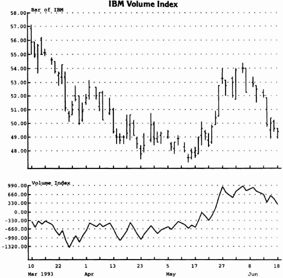
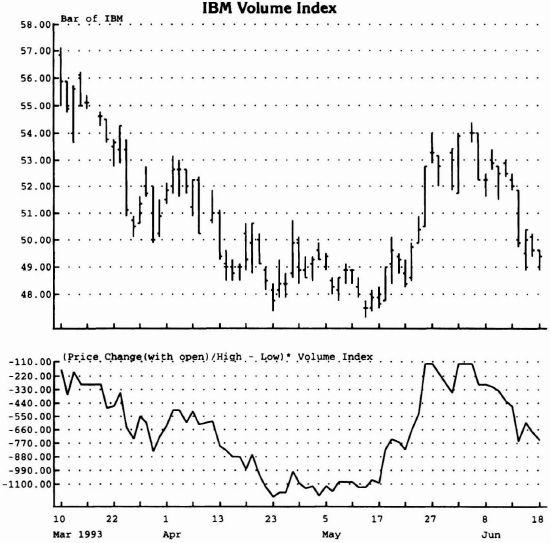
One simple technique developed to detect the basic trend merely involves the summation of daily volume; for example, if the closing price for the day is up, a positive value for that day is added to the cumulative total. Conversely, if the closing price for the day is down, a negative value for that day is added to the cumulative total. The index created is compared to the actual daily price movement, and divergences are identified to forecast price flow (see Figure 5.1).
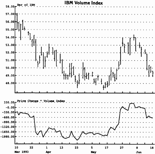
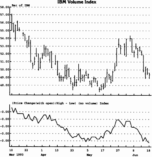
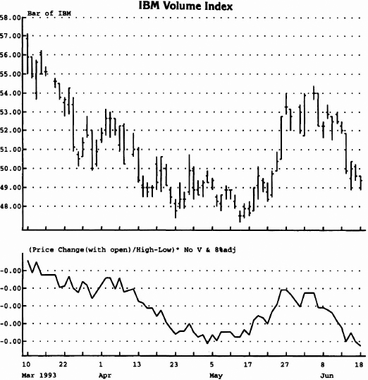
Another, more complicated method analyzes each transaction (tick) and continuously recalculates the index by multiplying the price change by the number of shares (contracts). Rather than scrutinizing each trade, however, other technicians isolate only the large-block (more than 10,000-share) transactions, assuming they are initiated by informed, sophisticated investors whose degree of aggressiveness is revealed by their price concessions. Other volume analysts rely on price change and volume, but merely compute their calculations daily at the conclusion of trading. They multiply the price change by the volume on that particular day to create an index (see Figure 5.2).
Source: Logical Information Machines, Inc. (LIM), Chicago, IL.
Figure 5.1 The concept behind this method is simple—volume precedes price movement. If the price close is up versus the previous day, accumulation is taking place. If the price close is down versus the previous day, distribution is dominant for that day. Practitioners of this method believe that, camouflaged behind seemingly random price movements, a cumulative index of accumulation and distribution will alert traders to the true market picture.
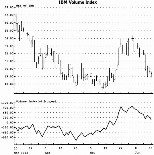
All these techniques were helpful, but none fulfilled my needs. I wanted something more exact and sensitive. A close friend and fellow market timer, Larry Williams, was working on precisely the same project. He convinced me that the proper reference point was the current day's open, rather than the previous day's closing price. Although all price services—whether presented dally in the newspaper or in other media sources, or obtained from quote machines—report price change from the previous day's close, this practice does not represent a true picture of price accumulation or distribution. It is not difficult to conclude that what occurred yesterday is history. Because of news events, the open could spike up or down and, consequently, a particular day's close could be higher than yesterday's close. As a result, what ostensibly appears to be accumulation or distribution based on the relationship of the current close versus the previous day's close would in actuality be precisely the opposite when compared to the same day's opening price (see Figure 5.3). Furthermore, to account for those exceptional cases when the open price is significantly different from the previous day's close, an adjustment formula can be inserted to account for the price gap and to deemphasize the movement from the current day's open and close.
Source: Logical Information Machines, Inc. (LIM), Chicago, IL.
Figure 5.2 By accounting for not only volume but also for the extent of the price movement (price concessions) from one close to the next, an index of accumulation–distribution can be enhanced.
Source: Logical Information Machines, Inc. (LIM), Chicago, IL.
Figure 5.3 What occurred yesterday is history. A more meaningful relationship than closing price movement is the relationship between a price close and that same day's opening price. If the close is greater than the open, accumulation has taken place; conversely, if the close is less than the open, distribution has taken place.
It was apparent that the current day's price range was a major component in measuring accumulation and distribution. By comparing the movement from the current day's close and open with that of the high to the low and by incorporating the factor of volume, a significant basis for a legitimate supply–demand model can be constructed. What I finally arrived at, however, was something considerably more complex and sensitive to shifts in supply and demand than this relatively crude approach. Specifically, although the relationship between price activity and the index was a good indicator of the direction of price, it was virtually impossible to compare the relative attractiveness of various securities because some issues were much more active (in volume) than others. Let me describe and explain in more detail how I was able to reconcile the issues of both comparing and ranking securities.
Just because I present my conclusions regarding the relationship between price change and volume, I do not mean to imply that my approach is necessarily the best; rather, it is the one I created and rely on after having researched and examined countless others. Its features are its logic, simplicity, and versatility, as well as its integration of numerous analytical approaches. Once mastered, it is designed to afford the user the ability to evaluate on a relative basis a large number of securities. Ideally, he will be able also to draw inferences regarding the cause of price advances or declines—was the rally the beginning of a sustained advance or just short covering? Rather than recite numerous other benefits derived from the techniques described herein, I will present them and highlight their advantages and disadvantages.
The techniques that follow are related, and the composite approach presented evolved over a period of many years. The creation of the nucleus was the most critical element in the process. Often, I challenged the logic and the foundation of my basic assumptions. Given what was available in the public domain, however, I was convinced that the basis was sufficiently sound to support all my derivative studies. As I discussed above, the critical item in distinguishing between accumulation (demand) and distribution (supply) is the reference point selected. Many years after I had concluded that the open was the proper pivot price for almost all measures of accumulation/distribution, I had this supposition confirmed by one of the major operators in the stock market. More specifically, everyone is aware of the stature and dominance assigned the specialists on the New York Stock Exchange. I had the pleasure of establishing a special kinship with one of the most respected of these individuals. I shared with him my theories and formulas regarding accumulation and distribution and the importance of the open price. He was amazed to learn of both my discoveries and my approach to analysis. He indicated to me that I had accomplished mathematically precisely what he had acquired intuitively over many years on the floor. To translate it into a workable code enabling an investor to monitor a large number of securities simultaneously was an effort he had previously believed unattainable. His endorsement reinforced my commitment to this method and further research.
Although the formulas are elementary, in order to fully appreciate their power and potential I recommend you experiment thoroughly with every facet of the concepts of accumulation/distribution presented (see Figure 5.4). The basis of all measures includes this formula:
![]()
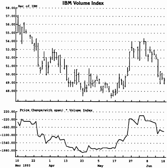
In other words, this calculation depicts the relationship of the close on a particular day to that day's open. If it is positive, it can be argued that price accumulation has taken place; if it is negative, price distribution has occurred. The intensity of the accumulation or distribution can be determined by relating movement from the open to the close, comparing it with the price range for that day (high to low), and then multiplying this ratio by that day's volume. In and of itself, this index value, when run cumulatively and compared with the underlying price activity, is a good indicator of future price movement.
Source: Logical Information Machines, Inc. (LIM), Chicago, IL.
Figure 5.4 By using the price change from close to open, as well as the volume, another index can be constructed.
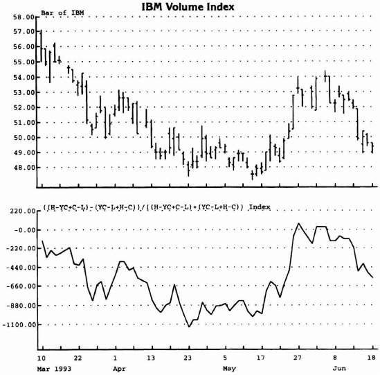
Before discussing the technique for standardizing securities, it is important to present an adjustment to this formula to compensate for significant opening price gaps of eight percent or more (see Figure 5.5). In these rare instances, even if price retraces back to the open, the exceptional inflation or deflation in the open price must be considered by introducing a formula that supersedes the original one. To calculate the buying (accumulation) pressure with an open or close of eight percent or greater than the previous day's close, the difference between today's high and yesterday's close is added to the difference between today's close and today's low. From this sum, the difference between today's high and today's close is subtracted. In turn, this value is divided by the difference between today's high and yesterday's close. The volume for the day is then multiplied by this value and added to the cumulative index. Conversely, in order to calculate the selling (distribution) pressure with an open eight percent or more less than the previous day's close, the difference between yesterday's close and today's low is added to the difference between today's high and today's close. From this sum, the difference between today's close and today's low is subtracted. In turn, this value is divided by the difference between yesterday's close and today's low. The volume for the day is then multiplied by this value and added to the cumulative index (see Figure 5.6).
Source: Logical Information Machines, Inc. (LIM), Chicago, IL.
Figure 5.5(a) By dividing the price movement from close to open by the price movement traversed for the entire day, the degree of aggressiveness is determined. For example, if price were to open on its low and close on its high on a particular day, it would suggest a more intensive buying campaign than if price were to open or close at the daily price midrange.
Source: Logical Information Machines, Inc. (LIM), Chicago, IL.
Figure 5.5(b) One chart [5-5(a)] illustrates with volume included and the other [5-5(b)] with no volume.
Source: Logical Information Machines, Inc. (LIM), Chicago, IL.
Figure 5.6 When an open occurs that is eight percent or more greater than or less than the previous day's close, an adjustment must be made to accentuate this atypical price behavior. Additionally, this formula can be used in lieu of opening prices when they are unavailable.
Should the open price be unobtainable for any reason, a version of the gap compensation formula would serve as a credible substitute. A few revisions are required, however:
- Calculate the difference between today's high and yesterday's close (if less than zero, then ignore) and the difference between today's close and today's low, to arrive at a measure of the buying pressure (buying pressure).
- Determine the difference between yesterday's close and today's low (if less than zero, then ignore), and add the difference between today's high and today's close (selling pressure).
- Add together the buying and selling pressure, and divide this value into the buying pressure figure if today is an up close; divide this value into the selling pressure if today is a down close.
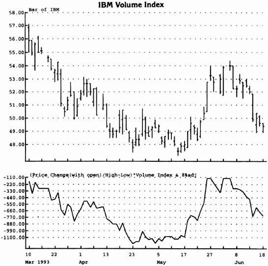
- Multiply this number by the total volume for the day and add to the cumulative index (see Figure 5.7a).
What you have learned so far are variations of what you may have already seen in the public domain. What I am about to share with you now is proprietary and essential to the task of comparing various securities to determine relative attractiveness. The concept is easy and straightforward, but it is important that you follow each step to ensure complete understanding and total mastery.
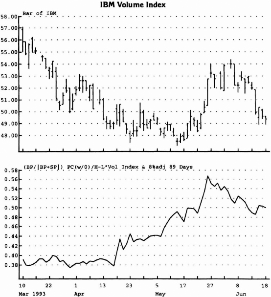
After the formula for calculating accumulation/distribution has been selected—I recommend the one using the open reference with the adjustment for open gaps of eight percent or more—a schedule of various time intervals is to be selected. I recommend an array of Fibonacci numbers beginning with five days and extending to 13, 21, 34, 55, 89, 144, 233, and 377 days. Each day, a value representing buying or selling pressure appears. Add together all the positive (buying pressure) numbers over the prescribed period of days, and then add together all the negative (selling pressure) numbers over that same period. Then divide the sum of all the buying pressure values by the absolute value of the sum of all the buying pressure values plus all the selling pressure values. This number is a ratio defining the buying pressure divided by the total activity (buying pressure plus selling pressure) and can be converted to a percentage by merely multiplying times 100 percent.
Source: Logical Information Machines, Inc. (LIM), Chicago, IL.
Figure 5.7(a) The adjustment for exceptional (eight percent or more) open gaps is introduced into the basic formula. Figure 5.7(a) includes volume.
In order to get the flavor of what is taking place within the dynamics of the market, this procedure can be applied to other time periods in the same manner. These percentages measure the demand over various time intervals, so it is possible to relate one security to another to determine which is being more aggressively accumulated or distributed. A chart of each security is even more helpful in displaying the movement of this oscillator (see Figure 5.8).
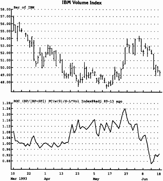
Even more important, however, is an indicator that displays the rate of change of the percentages. In fact, my experience has proven this value to be the most reliable in identifying attractive investment opportunities. The rate of change is calculated easily: divide the current day's percentage by the percentage X days ago. I typically work with Fibonacci numbers. Once a particular number is selected. I calculate the rate of change by dividing the value that day by the value at least four Fibonacci levels lower. For example, if I employ an 89-day series, to calculate the rate of change I would compare today's value with that of 13 days ago—in the Fibonacci series, 13 increases next to 21, 34, 55, then 89. As you can see, 13 is positioned four degrees beneath 89. If one were to use a 144-day series, then a comparison between the current day's value and that 21 days ago would be used; if one were to use a 233-day series, then a comparison between that day's value and the value 34 days earlier would be selected. Keep in mind that these are merely suggestions. You may have greater success at using other number series or comparing other periods of rates of change. Once selected, however, the period should remain static for all securities compared. For example, if an 89-day value is used for one stock and the rate of change is based on the value 13 days prior, then the same time periods should be used when evaluating the relative appeal of other stock candidates (see Figure 5.9). Once a value is selected, the index for most stocks will move within the same band. Experimentation with that index will yield the parameters associated with price tops and bottoms. Generally, the rate of change of this index will reverse prior to the actual price turns. Together with other techniques, entry and exit prices can be identified and the relative attraction of a situation can be compared with other opportunities.
Source: Logical Information Machines, Inc. (LIM), Chicago, IL.
Figure 5.7(b) This chart does not include volume.
Source: Logical Information Machines, Inc. (LIM), Chicago, IL.
Figure 5.8 It has always been difficult to relate the attractiveness of one security versus another. By calculating the percentage of buying pressure divided by the total pressure (both buying and selling), comparisons can be made. This measure is a serious breakthrough in trading analytics.
Source: Logical Information Machines, Inc. (LIM), Chicago, IL.
Figure 5.9 By determining the rate of change of buying pressure divided by the total pressure (both buying and selling), the degree of aggressiveness among various securities, as well as for individual securities, can be measured.
Source: Logical Information Machines, Inc. (LIM), Chicago, IL.
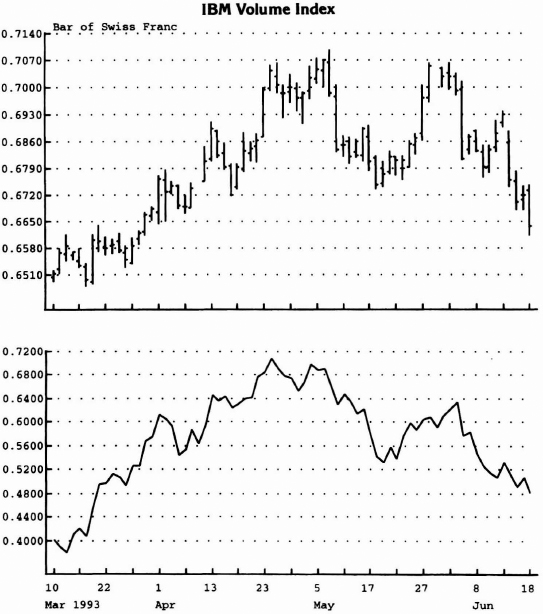
Figure 5.10 No volume and a different time period (34 days versus 34 days 5 days ago) are presented on this chart.
The above technique describes an accumulation/distribution model for stocks. The same approach can be applied to futures, with one exception. Whereas stocks have no restrictions as to the upside or downside movement they can traverse daily, futures have prescribed daily price limits because of the extreme leverage involved in those markets. When price moves limit, trading is virtually suspended. Although transactions can be effected at those price extremes, depending on the pool size looking to buy or sell, the volume the market is capable of producing may be significantly less than if there were no price limits. To account for this pent-up supply or demand, I recommend combining all consecutive days extending from the first day a limit move occurs until the last day of the series. The open price of the first day and the closing price of the last day, as well as the range and the volume for the entire period, are treated as if they were one day. This method incorporates the basic approach described and compensates for the shortcoming associated with limit moves. Some success is derived by excluding volume totally and running the formula described in Figure 5.9 with various other time periods both long and short term (see Figure 5.10).
As you can see, the model just described has application to both equities and futures. Variations of this model have equal application to these same markets with similar results. As with every other technique presented in this book, the best results are realized in combination with other proven approaches, thus enhancing the prospects of trading success. Consequently, my recommendation is not only to experiment and to introduce the accumulation/distribution model into your trading tool kit but also to utilize other methods that confirm your trading rules.