5
COMPUTER ARCHITECTURE

Chapter 4 walked through the design of a simple computer system and discussed how the CPU communicates with memory and I/O devices over the address and data buses. That’s not the end of the story, however. Many improvements over the years have made computers run faster while requiring less power and being easier to program. These improvements have added a lot of complexity to the designs.

Computer architecture refers to the arrangement of the various components into a computer—not to whether the box has Doric or Ionic columns or a custom shade of beige like the one American entrepreneur Steve Jobs (1955–2011) created for the original Macintosh computer. Many different architectures have been tried over the years. What’s worked and what hasn’t makes for fascinating reading, and many books have been published on the subject.

This chapter focuses primarily on architectural improvements involving memory. A photomicrograph of a modern microprocessor shows that the vast majority of the chip area is dedicated to memory handling. It’s so important that it deserves a chapter of its own. We’ll also touch on a few other differences in architectures, such as instruction set design, additional registers, power control, and fancier execution units. And we’ll discuss support for multitasking, the ability to run multiple programs simultaneously, or at least to provide the illusion of doing so. Running multiple programs implies the existence of some sort of supervisory program called an operating system (OS) that controls their execution.

Basic Architectural Elements

The two most common architectures are the von Neumann (named after Hungarian-American wizard John von Neumann, 1903–1957) and the Harvard (named after the Harvard Mark I computer, which was, of course, a Harvard architecture machine). We’ve already seen the parts; Figure 5-1 shows how they’re organized.

Figure 5-1: The von Neumann and Harvard architectures

Notice that the only difference between them is the way the memory is arranged. All else being equal, the von Neumann architecture is slightly slower because it can’t access instructions and data at the same time, since there’s only one memory bus. The Harvard architecture gets around that but requires additional hardware for the second memory bus.

Processor Cores

Both architectures in Figure 5-1 have a single CPU, which, as we saw in Chapter 4, is the combination of the ALU, registers, and execution unit. Multiprocessor systems with multiple CPUs debuted in the 1980s as a way to get higher performance than could be achieved with a single CPU. As it turns out, though, it’s not that easy. Dividing up a single program so that it can be parallelized to make use of multiple CPUs is an unsolved problem in the general case, although it works well for some things such as particular types of heavy math. However, it’s useful when you’re running more than one program at the same time and was a lifesaver in the early days of graphical workstations, as the X Window System was such a resource hog that it helped to have a separate processor to run it.

Decreasing fabrication geometries lowers costs. That’s because chips are made on silicon wafers, and making things smaller means more chips fit on one wafer. Higher performance used to be achieved by making the CPU faster, which meant increasing the clock speed. But faster machines required more power, which, combined with smaller geometries, produced more heat-generating power per unit of area. Processors hit the power wall around 2000 because the power density couldn’t be increased without exceeding the melting point.

Salvation of sorts was found in the smaller fabrication geometries. The definition of CPU has changed; what we used to call a CPU is now called a processor core. Multicore processors are now commonplace. There are even systems, found primarily in data centers, with multiple multicore processors.

Microprocessors and Microcomputers

Another orthogonal architectural distinction is based on mechanical packaging. Figure 5-1 shows CPUs connected to memory and I/O. When the memory and I/O are not in the same physical package as the processor cores, we call it a microprocessor, whereas when everything is on a single chip, we use the term microcomputer. These are not really well-defined terms, and there is a lot of fuzziness around their usage. Some consider a microcomputer to be a computer system built around a microprocessor and use the term microcontroller to refer to what I’ve just defined as a microcomputer.

Microcomputers tend to be less powerful machines than microprocessors because things like on-chip memory take a lot of space. We’re not going to focus on microcomputers much in this chapter because they don’t have the same complexity of memory issues. However, once you learn to program, it is worthwhile to pick up something like an Arduino, which is a small Harvard architecture computer based on an Atmel AVR microcomputer chip. Arduinos are great for building all sorts of toys and blinky stuff.

To summarize: microprocessors are usually components of larger systems, while microcomputers are what you find in things like your dishwasher.

There’s another variation called a system on a chip (SoC). A passable but again fuzzy definition is that a SoC is a more complex microcomputer. Rather than having relatively simple on-chip I/O, a SoC can include things like Wi-Fi circuitry. SoCs are found in devices such as cell phones. There are even SoCs that include field-programmable gate arrays (FPGAs), which permit additional customization.

Procedures, Subroutines, and Functions

Many engineers are afflicted with a peculiar variation of laziness. If there’s something they don’t want to do, they’ll put their energy into creating something that does it for them, even if that involves more work than the original task. One thing programmers want to avoid is writing the same piece of code more than once. There are good reasons for that besides laziness. Among them is that it makes the code take less space and, if there is a bug in the code, it only has to be fixed in one place.

The function (or procedure or subroutine) is a mainstay of code reuse. Those terms all mean the same thing as far as you’re concerned; they’re just regional differences in language. We’ll use function because it’s the most similar to what you may have learned in math class.

Most programming languages have similar constructs. For example, in JavaScript we could write the code shown in Listing 5-1.

function
cube(x)
{
        return (x * x * x);
}

Listing 5-1: A sample JavaScript function

This code creates a function named cube that takes a single parameter named x and returns its cube. Keyboards don’t include the multiplication (×) symbol, so many programming languages use * for multiplication instead. Now we can write a program fragment like Listing 5-2.

y = cube(3);

Listing 5-2: A sample JavaScript function call

The nice thing here is that we can invoke, or call, the cube function multiple times without having to write it again. We can find cube(4) + cube(6) without having to write the cubing code twice. This is a trivial example, but think about how convenient this capability would be for more complicated chunks of code.

How does this work? We need a way to run the function code and then get back to where we were. To get back, we need to know where we came from, which is the contents of the program counter (which you saw back in Figure 4-12 on page 101). Table 5-1 shows how to make a function call using the example instruction set we looked at in “Instruction Set” on page 102.

Table 5-1: Making a Function Call

Address	Instruction	Operand	Comments
100	pca		Program counter → accumulator
101	add	5 (immediate)	Address for return (100 + 5 = 105)
102	store	200 (direct)	Store return address in memory
103	load	3 (immediate)	Put number to cube (3) in accumulator
104	bra	300 (direct)	Call the cube function
105			Continues here after function
...
200			Reserved memory location
...
300	...	...	The cube function
...			Remainder of cube function
310	bra	200 (indirect)	Branch to stored return address

What’s happening here? We first calculate the address of where we want execution to continue after returning from the cube function. It takes us a few instructions to do that; plus, we need to load the number that must be cubed. That’s five instructions later, so we store that address in memory location 200. We branch off to the function, and when the function is done, we branch indirect through 200, so we end up at location 105. This process plays out as shown in Figure 5-2.

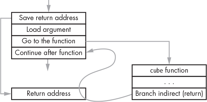
Figure 5-2: A function call flow

This is a lot of work for something that is done a lot, so many machines add helper instructions. For example, ARM processors have a Branch with Link (BL) instruction that combines the branch to the function with saving the address of the following instruction.

Stacks

Functions aren’t limited to simple pieces of code such as the example we just saw. It’s common for functions to call other functions and for them to call themselves.

Wait, what was that? A function calling itself? That’s called recursion, and it’s really useful. Let’s look at an example. Your phone probably uses JPEG (Joint Photographic Experts Group) compression to reduce the file size of photos. To see how compression works, let’s start with a square black-and-white image, shown in Figure 5-3.

Figure 5-3: A crude smiley face

We can attack the compression problem using recursive subdivision: we look at the image, and if it’s not all one color, we divide it into four pieces, then check again, and so on until the pieces are one pixel in size.

Listing 5-3 shows a subdivide function that processes a portion of the image. It’s written in pseudocode, an English-like programming language made up for examples. It takes the x- and y-coordinates of the lower-left corner of a square along with the size (we don’t need both the width and the height, since the image is a square). “Takes” is just shorthand for what’s called the arguments to a function in math.

function
subdivide(x, y, size)
{
    IF (size ≠ 1 AND the pixels in the square are not all the same color) {
        half = size ÷ 2
        subdivide(x, y, half) lower          left quadrant
        subdivide(x, y + half, half)         upper left quadrant
        subdivide(x + half, y + half, half)  upper right quadrant
        subdivide(x + half, y, half)         lower right quadrant
    }
    ELSE {
        save the information about the square
    }
}

Listing 5-3: A subdivision function

The subdivide function partitions the image into same-colored chunks starting with the lower-left quadrant, then the upper left, upper right, and finally the lower right. Figure 5-4 shows things that need subdividing in gray and things that are solidly one color in black or white.

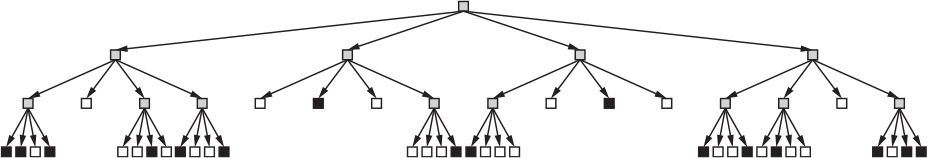
Figure 5-4: Subdividing the image

What we have here looks like what computer geeks call a tree and what math geeks call a directed acyclic graph (DAG). You follow the arrows. In this structure, arrows don’t go up, so there can’t be loops. Things with no arrows going out of them are called leaf nodes, and they’re the end of the line, like leaves are the end of the line on a tree branch. If you squint enough and count them in Figure 5-4, you can see that there are 40 solid squares, which is fewer than the 64 squares in the original image, meaning there’s less information to store. That’s compression.

For some reason, probably because it’s easier to draw (or maybe because they rarely go outside), computer geeks always put the root of the tree at the top and grow it downward. This particular variant is called a quadtree because each node is divided into four parts. Quadtrees are spatial data structures. Hanan Samet has made these his life’s work and has written several excellent books on the subject.

There’s a problem with implementing functions as shown in the previous section. Because there’s only one place to store the return value, functions like this can’t call themselves because that value would get overwritten and we’d lose our way back.

We need to be able to store multiple return addresses in order to make recursion work. We also need a way to associate the return addresses with their corresponding function calls. Let’s see if we can find a pattern in how we subdivided the image. We went down the tree whenever possible and only went across when we ran out of downward options. This is called a depth-first traversal, as opposed to going across first and then down, which is a breadth-first traversal. Every time we go down a level, we need to remember our place so that we can go back. Once we go back, we no longer need to remember that place.

What we need is something like those gadgets that hold piles of plates in a cafeteria. When we call a function, we stick the return address on a plate and put it on top of the pile. When we return from the call, we remove that plate. In other words, it’s a stack. You can sound important by calling it a LIFO (“last in, first out”) structure. We push things onto the stack, and pop them off. When we try to push things onto a stack that doesn’t have room, that’s called a stack overflow. Trying to pop things from an empty stack is a stack underflow.

We can do this in software. In our earlier function call example in Table 5-1, every function could take its stored return address and push it onto a stack for later retrieval. Fortunately, most computers have hardware support for stacks because they’re so important. This support includes limit registers so that the software doesn’t have to constantly check for possible overflow. We’ll talk about how processors handle exceptions, such as exceeding limits, in the next section.

Stacks aren’t just used for return addresses. Our subdivide function included a local variable where we calculated half the size once and then used it eight times to make the program faster. We can’t just overwrite this every time we call the function. Instead, we store local variables on the stack too. That makes every function call independent of other function calls. The collection of things stored on the stack for each call is a stack frame. Figure 5-5 illustrates an example from our function in Listing 5-3.

Figure 5-5: Stack frames

We follow the path shown by the heavy black squares. You can see that each call generates a new stack frame that includes both the return address and the local variable.

Several computer languages, such as forth and PostScript, are stack-based (see “Different Equation Notations”), as are several classic HP calculators. Stacks aren’t restricted to just computer languages, either. Japanese is stack-based: nouns get pushed onto the stack and verbs operate on them. Yoda’s cryptic utterances also follow this pattern.

Interrupts

Imagine that you’re in the kitchen whipping up a batch of chocolate chip cookies. You’re following a recipe, which is just a program for cooks. You’re the only one home, so you need to know if someone comes to the door. We’ll represent your activity using a flowchart, which is a type of diagram used to express how things work, as shown in Figure 5-6.

Figure 5-6: Home alone making cookies #1

This might work if someone really patient comes to the door. But let’s say that a package is being delivered that needs your signature. The delivery person isn’t going to wait 45 minutes, unless they can smell the cookies and are hoping to get some. Let’s try something different, like Figure 5-7.

Figure 5-7: Home alone making cookies #2

This technique is called polling. It works, but not very well. You’re less likely to miss your delivery, but you’re spending a lot of time checking the door.

We could divide up each of the cookie-making tasks into smaller subtasks and check the door in between them. That would improve your chances of receiving the delivery, but at some point you’d be spending more time checking the door than making cookies.

This is a common and important problem for which there is really no software solution. It’s not possible to make this work well by rearranging the structure of a program. What’s needed is some way to interrupt a running program so that it can respond to something external that needs attention. It’s time to add some hardware features to the execution unit.

Pretty much every processor made today includes an interrupt unit. Usually it has pins or electrical connections that generate an interrupt when wiggled appropriately. Pin is a colloquial term for an electrical connection to a chip. Chips used to have parts that looked like pins, but as devices and tools have gotten smaller, many other variants have emerged. Many processor chips, especially microcomputers, have integrated peripherals (on-chip I/O devices) that are connected to the interrupt system internally.

Here’s how it works. A peripheral needing attention generates an interrupt request. The processor (usually) finishes up with the currently executing instruction. It then puts the currently executing program on hold and veers off to execute a completely different program called an interrupt handler. The interrupt handler does whatever it needs to do, and the main program continues from where it left off. Interrupt handlers are functions.

The equivalent mechanism for the cookie project is a doorbell. You can happily make cookies until you’re interrupted by the doorbell, although it can be annoying to be interrupted by pollsters. There are a few things to consider. First is your response time to the interrupt. If you spend a long time gabbing with the delivery person, your cookies may burn; you need to make sure that you can service interrupts in a timely manner. Second, you need some way to save your state when responding to an interrupt so that you can go back to whatever you were doing after servicing it. For example, if the interrupted program had something in a register, the interrupt handler must save the contents of that register if it needs to use it and then restore it before returning to the main program.

The interrupt system uses a stack to save the place in the interrupted program. It is the interrupt handler’s job to save anything that it might need to use. This way, the handler can save the absolute minimum necessary so that it works fast.

How does the computer know where to find the interrupt handler? Usually, there’s a set of reserved memory addresses for interrupt vectors, one for each supported interrupt. An interrupt vector is just a pointer, the address of a memory location. It’s similar to a vector in math or physics—an arrow that says, “Go there from here.” When an interrupt occurs, the computer looks up that address and transfers control there.

Many machines include interrupt vectors for exceptions including stack overflow and using an invalid address such as one beyond the bounds of physical memory. Diverting exceptions to an interrupt handler often allows the interrupt handler to fix problems so that the program can continue running.

Typically, there are all sorts of other special interrupt controls, such as ways to turn specific interrupts on and off. There is often a mask so that you can say things like “hold my interrupts while the oven door is open.” On machines with multiple interrupts, there is often some sort of priority ordering so that the most important things get handled first. That means that the handlers for lower-priority interrupts may themselves be interrupted. Most machines have one or more built-in timers that can be configured to generate interrupts.

Operating systems, discussed in the next section, often keep access to the physical (hardware) interrupts out of reach from most programs. They substitute some sort of virtual or software interrupt system. For example, the UNIX operating system has a signal mechanism. More recently developed systems call these events.

Relative Addressing

What would it take to have multiple programs running at the same time? For starters, we’d have to have some sort of supervisor program that knew how to switch between them. We’ll call this program an operating system or operating system kernel. We’ll make a distinction between the OS and the programs it supervises by calling the OS a system program and everything else user programs, or processes. A simple OS might work something like Figure 5-8.

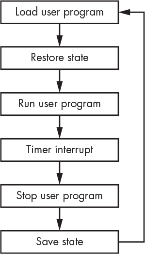
Figure 5-8: A simple operating system

The OS here is using a timer to tell it when to switch between user programs. This scheduling technique is called time slicing because it gives each program a slice of time in which to run. The user program state or context refers to the contents of the registers and any memory that the program is using, including the stack.

This works, but it’s pretty slow. It takes time to load a program. It would be much faster if you could load the programs into memory as space allows and keep them there, as shown in Figure 5-9.

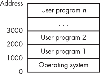
Figure 5-9: Multiple programs in memory

In this example, user programs are loaded into memory one after another. But wait, how can this work? As explained back in “Addressing Modes” on page 104, our sample computer used absolute addressing, which means that the addresses in the instructions referred to specific memory locations. It’s not going to work to run a program that expects to be at address 1000 at a different address, such as 2000.

Some computers solve this problem by adding an index register (Figure 5-10). This is a register whose contents are added to addresses to form effective addresses. If a user program expects to be run at address 1000, the OS could set the index register to 2000 before running it at address 3000.

Figure 5-10: An index register

Another way to fix this is with relative addressing—which is not about sending a birthday card to your auntie. Instead of the addresses in instructions being relative to 0 (the beginning of memory in most machines), they can be relative to the address of their instruction. Go back and review Table 4-4 on page 108. You can see that the second instruction contains the address 100 (110100 in binary). With relative addressing, that would become +99, since the instruction is at address 1 and address 100 is 99 away. Likewise, the last instruction is a branch to address 4, which would become a branch to –8 with relative addressing. This sort of stuff is a nightmare to do in binary, but modern language tools do all the arithmetic for us. Relative addressing allows us to relocate a program anywhere in memory.

Memory Management Units

Multitasking has evolved from being a luxury to being a basic requirement now that everything is connected to the internet, because communications tasks are constantly running in the background—that is, in addition to what the user is doing. Index registers and relative addressing help, but they’re not enough. What happens if one of these programs contains bugs? For example, what if a bug in user program 2 (Figure 5-9) causes it to overwrite something in user program 1—or even worse, in the OS? What if someone deliberately wrote a program to spy on or change other programs running on the system? We’d really like to isolate each program to make those scenarios impossible. To that end, most microprocessors now include memory management unit (MMU) hardware that provides this capability. MMUs are very complicated pieces of hardware.

Systems with MMUs make a distinction between virtual addresses and physical addresses. The MMU translates the virtual addresses used by programs into physical addresses used by memory, as shown in Figure 5-11.

Figure 5-11: MMU address translation

How is this different from an index register? Well, there’s not just one. And the MMUs aren’t the full width of the address. What’s happening here is that we’re splitting the virtual address into two parts. The lower part is identical to the physical address. The upper part undergoes translation via a piece of RAM called the page table, an example of which you can see in Figure 5-12.

Memory is partitioned into 256-byte pages in this example. The page table contents control the actual location of each page in physical memory. This allows us to take a program that expects to start at address 1000 and put it at 2000, or anywhere else as long as it’s aligned on a page boundary. And although the virtual address space appears continuous to the program, it does not have to be mapped to contiguous physical memory pages. We could even move a program to a different place in physical memory while it’s running. We can provide one or more cooperating programs with shared memory by mapping portions of their virtual address space to the same physical memory. Note that the page table contents become part of a program’s context.

Figure 5-12: Simple page table for a 16-bit machine

Now, if you’ve been paying attention, you might notice that the page table just looks like a piece of memory. And you’d be correct. And you’d expect me to tell you that it’s not that simple. Right again.

Our example uses 16-bit addresses. What happens if we have a modern machine with 64-bit addresses? If we split the address in half, we need 4 GiB of page table, and the page size would also be 4 GiB—not very useful since that’s more memory than many systems have. We could make the page size smaller, but that would increase the page table size. We need a solution.

The MMU in a modern processor has a limited page table size. The complete set of page table entries is kept in main memory, or on disk if memory runs out. The MMU loads a subset of the page table entries into its page table as needed.

Some MMU designs add further control bits to their page tables—for example, a no-execute bit. When this bit is set on a page, the CPU won’t execute instructions from that page. This prevents programs from executing their own data, which is a security risk. Another common control bit makes pages read only.

MMUs generate a page fault exception when a program tries to access an address that isn’t mapped to physical memory. This is useful, for example, in the case of stack overflow. Rather than having to abort the running program, the OS can have the MMU map some additional memory to grow the stack space and then resume the execution of the user program.

MMUs make the distinction between von Neumann and Harvard architectures somewhat moot. Such systems have the single bus of the von Neumann architecture but can provide separate instruction and data memory.

Virtual Memory

Operating systems manage the allocation of scarce hardware resources among competing programs. For example, we saw an OS manage access to the CPU itself in Figure 5-8. Memory is also a managed resource. Operating systems use MMUs to provide virtual memory to user programs.

We saw earlier that the MMU can map a program’s virtual addresses to physical memory. But virtual memory is more than that. The page fault mechanism allows programs to think that they can have as much memory as they want, even if that exceeds the amount of physical memory. What happens when the requested memory exceeds the amount available? The OS moves the contents of memory pages that aren’t currently needed out to larger but slower mass storage, usually a disk. When a program tries to access memory that has been swapped out, the OS does whatever it needs to in order to make space and then copies the requested page back in. This is known as demand paging. Figure 5-13 shows a virtual memory system with one page swapped out.

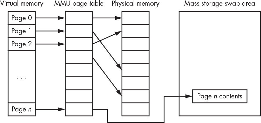
Figure 5-13: Virtual memory

System performance takes a big hit when swapping occurs, but it’s still better than not being able to run a program at all because of insufficient memory. Virtual memory systems use a number of tricks to minimize the performance hit. One of these is a least recently used (LRU) algorithm that tracks accesses to pages. The most frequently used pages are kept in physical memory; the least recently used are swapped out.

System and User Space

Multitasking systems give each process the illusion that it’s the only program running on the computer. MMUs help to foster this illusion by giving each process its own address space. But this illusion is difficult to maintain when it comes to I/O devices. For example, the OS uses a timer device to tell it when to switch between programs in Figure 5-8. The OS decides to set the timer to generate an interrupt once per second, but if one of the user programs changes it to interrupt once per hour, things won’t work as expected. Likewise, the MMU wouldn’t provide any serious isolation between programs if any user program could modify its configuration.

Many CPUs include additional hardware that addresses this problem. There is a bit in a register that indicates whether the computer is in system or user mode. Certain instructions, such as those that deal with I/O, are privileged and can be executed only in system mode. Special instructions called traps or system calls allow user mode programs to make requests of system mode programs, which means the operating system.

This arrangement has several advantages. First, it protects the OS from user programs and user programs from each other. Second, since user programs can’t touch certain things like the MMU, the OS can control resource allocation to programs. System space is where hardware exceptions are handled.

Any programs that you write for your phone, laptop, or desktop will run in user space. You need to get really good before you touch programs running in system space.

Memory Hierarchy and Performance

Once upon a time, CPUs and memory worked at the same speed, and there was peace in the land. However, CPUs got faster and faster, and although memory got faster too, it couldn’t keep up. Computer architects have come up with all sorts of tricks to make sure that those fast CPUs aren’t sitting around waiting for memory.

Virtual memory and swapping introduce the notion of memory hierarchy. Although all memory looks the same to a user program, what happens behind the scenes greatly affects the system performance. Or, to paraphrase George Orwell, all memory accesses are equal, but some memory accesses are more equal than others.

Computers are fast. They can execute billions of instructions per second. But not much would get done if the CPU had to wait around for those instructions to arrive, or for data to be retrieved or stored.

We’ve seen that processors include some very fast, expensive memory called registers. Early computers had only a handful of registers, whereas some modern machines contain hundreds. But overall, the ratio of registers to memory has gotten smaller. Processors communicate with main memory, usually DRAM, which is less than a tenth as fast as the processor. Mass storage devices such as disk drives may be a millionth as fast the processor.

Time for a food analogy courtesy of my friend Clem. Registers are like a refrigerator: there’s not a lot of space in there, but you can get to its contents quickly. Main memory is like a grocery store: it has a lot more space for stuff, but it takes a while to get there. Mass storage is like a warehouse: there’s even more space for stuff, but it’s much farther away.

Let’s milk this analogy some more. You often hit the fridge for one thing. When you make the trip to the store, you fill a few grocery bags. The warehouse supplies the store by the truckload. Computers are the same way. Small blocks of stuff are moved between the CPU and main memory. Larger blocks of stuff are moved between main memory and the disk. Check out The Paging Game by Jeff Berryman for a humorous explanation of how all this works.

Skipping a lot of gory details, let’s assume the CPU runs about 10 times the speed of main memory. That translates to a lot of time spent waiting for memory, so additional hardware (faster on-chip memory) was added for a pantry or cache. It’s much smaller than the grocery store, but much faster when running at full processor speed.

How do we fill the pantry from the grocery store? Way back in “Random-Access Memory” on page 82, we saw that DRAM performs best when accessing columns out of a row. When you examine the way programs work, you notice that they access sequential memory locations unless they hit a branch. And a fair amount of the data used by a program tends to clump together. This phenomenon is exploited to improve system performance. The CPU memory controller hardware fills the cache from consecutive columns in a row because, more often than not, data is needed from sequential locations. Rather than getting one box of cereal, we put several in sacks and bring them home. By using the highest-speed memory-access mode available, CPUs are usually ahead of the game even when there is a cache miss caused by a nonsequential access. A cache miss is not a contestant in a Miss Cache pageant; it’s when the CPU looks for something in the cache that isn’t there and has to fetch it from memory. Likewise, a cache hit is when the CPU finds what it’s looking for in the cache. You can’t have too much of a good thing.

There are several levels of cache memory, and they get bigger and slower as they get farther away from the CPU (even when they’re on the same chip). These are called the L1, L2, and L3 caches, where the L stands for level. Yup, there’s the spare freezer in the garage plus the storeroom. And there’s a dispatcher that puts air traffic control to shame. There’s a whole army of logic circuitry whose job it is to pack and unpack grocery bags, boxes, and trucks of different sizes to make all this work. It actually takes up a good chunk of the chip real estate. The memory hierarchy is outlined in Figure 5-14.

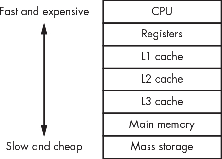
Figure 5-14: Memory hierarchy

Additional complicated tweaks have improved performance even further. Machines include branch prediction circuitry that guesses the outcome of conditional branch instructions so that the correct data can be prefetched from memory and in the cache ready to go. There is even circuitry to handle out-of-order execution. This allows the CPU to execute instructions in the most efficient order even if it’s not the order in which they occur in a program.

Maintaining cache coherency is a particularly gnarly problem. Imagine a system that contains two processor chips, each with four cores. One of those cores writes data to a memory location—well, really to a cache, where it will eventually get into memory. How does another core or processor know that it’s getting the right version of the data from that memory location? The simplest approach is called write through, which means that writes go directly to memory and are not cached. But that eliminates many of the benefits of caching, so there’s a lot of additional cache-management hardware for this that is outside of the scope of this book.

Coprocessors

A processor core is a pretty complicated piece of circuitry. You can free up processor cores for general computation by offloading common operations to simpler pieces of hardware called coprocessors. It used to be that coprocessors existed because there wasn’t room to fit everything on a single chip. For example, there were floating-point coprocessors for when there wasn’t space for floating-point instruction hardware on the processor itself. Today there are on-chip coprocessors for many things, including specialized graphics processing.

In this chapter we’ve talked about loading programs into memory to be run, which usually means that the programs are coming from some slow and cheap memory, such as a disk drive. And we’ve seen that virtual memory systems may be reading from and writing to disks as part of swapping. And we saw in “Block Devices” on page 85 that disks aren’t byte-addressable—they transfer blocks of 512 or 4,096 bytes. This means there’s a lot of copying between main memory and disk that’s straightforward, because no other computation is needed. Copying data from one place to another is one of the biggest consumers of CPU time. Some coprocessors do nothing but move data around. These are called direct memory access (DMA) units. They can be configured to do operations like “move this much stuff from here to there and let me know when you’re done.” CPUs offload a lot of grunt work onto DMA units, leaving the CPU free to do more useful operations.

Arranging Data in Memory

We learned from the program in Table 4-4 that memory is used not only for the instructions but for data as well. In this case, it’s static data, meaning that the amount of memory needed is known when the program is written. We saw earlier in this chapter that programs also use memory for stacks. These data areas need to be arranged in memory so that they don’t collide.

Figure 5-15 illustrates the typical arrangement for both von Neumann and Harvard architecture machines without MMUs. You can see that the only difference is that instructions reside in separate memory on Harvard architecture machines.

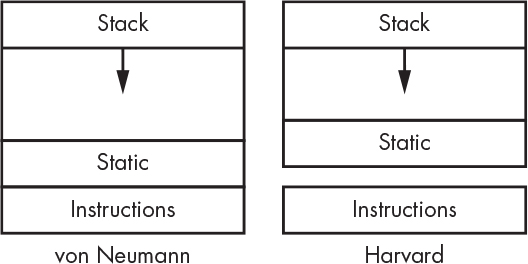
Figure 5-15: Memory arrangement

There’s one more way in which programs use memory. Most programs have to deal with dynamic data, which has a size that is unknown until the program is running. For example, an instant messaging system doesn’t know in advance how many messages it needs to store or how much storage will be needed for each message. Dynamic data is customarily piled into memory above the static area, called the heap, as shown in Figure 5-16. The heap grows upward as more space is needed for dynamic data, while the stack grows downward. It’s important to make sure they don’t collide. There are a few minor variations on this theme; some processors reserve memory addresses at the beginning or end of memory for interrupt vectors and registers that control on-chip I/O devices.

Figure 5-16: Memory arrangement with the heap

You’ll find this memory layout when using microcomputers, as they typically don’t have MMUs. When MMUs are involved, the instructions, data, and stack are mapped to different physical memory pages whose size can be adjusted as needed. But the same memory layout is used for the virtual memory presented to programs.

Running Programs

You’ve seen that computer programs have a lot of pieces. In this section, you’ll learn how they all come together.

Earlier I said that programmers use functions for code reuse. That’s not the end of the story. There are many functions that are useful for more than one program—for example, comparing two text strings. It would be nice if we could just use these third-party functions rather than having to write our own every time. One way to do that is by grouping related functions into libraries. There are a large number of libraries available for everything from string handling to hairy math to MP3 decoding.

In addition to libraries, nontrivial programs are usually built in pieces. Though you could put the entirety of a program into a single file, there are several good reasons to break it up. Chief among these is that it makes it easier for several people to work on the same program at the same time.

But breaking programs up means we need some way to hook or link all the different pieces together. The way we accomplish this is by processing each program piece into an intermediate format designed for this purpose and then running a special linker program that makes all the connections. Many intermediate file formats have been developed over the years. Executable and Linkable Format (ELF) is currently the most popular flavor. This format includes sections similar to want ads. There might be something in the For Sale section that says, “I have a function named cube.” Likewise, we might see “I’m looking for a variable named date” in the Wanted section.

A linker is a program that resolves all the ads, resulting in a program that can actually be run. But of course, there are complications in the name of performance. It used to be that you treated libraries just like one of your files full of functions and linked them in with the rest of your program. This was called static linking. Sometime in the 1980s, however, people noticed that lots of programs were using the same libraries. This was a great testament to the value of those libraries. But they added to the size of every program that used them, and there were many copies of the libraries using up valuable memory. Enter shared libraries. The MMU can be used to allow the same copy of a library to be shared by multiple programs, as illustrated in Figure 5-17.

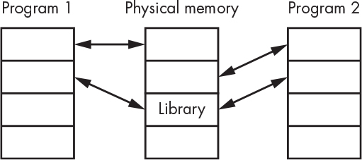
Figure 5-17: A shared library

Keep in mind that the instructions from the shared library are common to the programs that use it. The library functions must be designed so that they use the heap and stack of the calling programs.

Programs have an entry point, which is the address of the first instruction in the program. Though it’s counterintuitive, that instruction is not the first one executed when a program is run. When all the pieces of a program are linked to form an executable, an additional runtime library is included. Code in this library runs before hitting the entry point.

The runtime library is responsible for setting up memory. That means establishing a stack and a heap. It also sets the initial values for items in the static data area. These values are stored in the executable and must be copied to the static data after acquiring that memory from the system.

The runtime library performs many more functions, especially for complicated languages. Fortunately, you don’t need to know any more about it right now.

Memory Power

We’ve approached memory from a performance perspective so far. But there’s another consideration. Moving data around in memory takes power. That’s not a big deal for desktop computers. But it’s a huge issue for mobile devices. And although battery life isn’t an issue in data centers such as those used by large internet companies, using extra power on thousands of machines adds up.

Balancing power consumption and performance is challenging. Keep both in mind when writing code.

Summary

You’ve learned that working with memory is not as simple as you might have thought after reading Chapter 4. You got a feel for how much additional complication gets added to simple processors in order to improve memory usage. You now have a pretty complete idea of what’s in a modern computer with the exception of I/O—which is the topic of Chapter 6.