
This chapter shows how you can spend less time tuning in a larger performance environment by first tuning in a modest-sized, smaller environment. In this smaller environment, you can complete more fix-test cycles per day, which greatly accelerates the overall tuning process.
The objectives of this chapter are:
- Learn how to design load tests that will run in a very small computing environment (like your desktop), effectively turning it into an economical performance tuning lab.
- Learn how to graph CPU/RAM consumption of individual processes over time.
- Learn how to replace back-end systems with a stub server that returns prerecorded responses.
Scheduling the performance-tuning phase of a project in the rough vicinity of a code freeze is a bad idea, but that is precisely where we schedule it. The code freezers say, “No more changes” and the tuners reply back, grunting “must fix code.” The argument ends in a slap fight outside on the playground next to the slide. This is productivity, SDLC-style
. Even after witnessing this entire kerfuffle, management can’t seem to figure out why system performance ends up being so awful. The perennial conflict between “code freeze” and “code change” goes unnoticed, again.
This chapter explores a set of techniques that will enable you to use a small, developer tuning environment to boost performance early and throughout the SDLC. A final performance vetting in a large, production-like environment will likely still be required, but the early vetting will keep it from devolving into a more traditional, angst-ridden rush-job crammed into the closing moments before production.
Rapid Tuning
Many will rightfully object that a small tuning environment with just a few CPUs is too small to meet final performance goals for a high-throughput system
. That is a fair objection. But reaching maximum throughput is not the immediate goal. Instead, the small environment provides an easy-to-access and easy-to-monitor system where we can complete many fix-test cycles, perhaps as many as 10 a day.
In a single fix-cycle, you run a load test for a few minutes, use monitoring tools to identify the biggest performance issue, code and deploy a code fix, validate the improvement, and then repeat.
Traditionally, after the code is finished and Quality Assurance has tested all the code, performance testing is tightly crammed into the schedule right before production. This is particularly challenging for a number reasons. First, there is so little time to create the expensive, large computing environment that most feel is required for tuning. Second, for stability’s sake, it makes sense to institute a code freeze as production draws near. However, the culture of the code freeze makes it particularly difficult for performance engineers to test and deploy the changes required to make the system perform. Lastly, there is little time to retreat from poorly performing technical approaches that were tightly baked into the product from day 1. This is a last minute rush-job.
To contrast, this “rapid tuning” approach helps keep tuning from consuming your budget and helps avoid a last-minute performance rush-job. With the bulk of the performance defects addressed early on, demonstrating the full throughput goal in the full environment is a smaller, more manageable task.
Write-Once-Run-Anywhere Performance Defects
The code samples that accompany this book are available in these two github repositories:
I’ll refer to the first one as “jpt” and the second one as “littleMock.” This section briefly enumerates the performance defects in the first set of examples—jpt. There is more detail on both sets of examples in Chapter 8. Chapters 1, 2, and 3 are introductory in nature, so I can understand why the hard performance data from load tests in Table 2-1 seems out of place. I have included this data to provide tangible proof that commonly found performance defects can be easily detected in a modest-sized tuning environment, like a workstation.
Table 2-1.
Throughput results from jpt Sample Performance Defects That You Can Run on Your Own Machine. RPM = Requsts per Minute, as measured by Glowroot.org.
Test # | A Test RPM | B Test RPM | Performance Defect | Comments |
|---|---|---|---|---|
01 | 119 | 394 | Slow HTTP back-end | |
02 | 2973 | 14000 | Multiple reads to 1MB data file | |
03 | 15269 | 10596 | Uncached queries to static data | |
04 | 6390 | 15313 | Slow result set iteration | |
05 | 3801 | 12 | Missing database index | |
06 | 10573 | 10101 | Over-allocation of RAM on heap | No significant throughput difference, but essential for avoiding waste. |
07 | 18150 | 26784 | SELECT N+1 | |
08 | 354 | 354 | Runaway thread with heavy CPU | Extra CPU consumption did not impact throughput. |
09 | N/A | N/A | Multiple Issues | 09b.jmx does not exist. Try this yourself. |
10 | N/A | N/A | Uncompressed HTTPS response over WAN | Results only interesting when tested over a WAN. |
11 | N/A | N/A | Memory leak | 11a throughput degrades, but only after the slow leak fills the heap. |
12 | 7157 | 9001 | Undersized Young Generation |
Each row in Table 2-1 details two tests—one with and the other without a particular performance defect. From row-to-row, it varies on whether the A or the B test has the defect. The test with the higher RPM has the better performance, although there are a few exceptions where other factors besides RPM determine best performance.
Like this set of examples, most performance defects are “Write-Once-Run-Anywhere” (WORA) defects
, because regardless of whether you run them on a massive, clustered environment or a small laptop, the defect will still be there and it will be detectable.
I don’t expect others to reproduce
the exact numbers that I’ve included in this table. Rather, the main idea is to understand that there are concrete and repeatable performance differences between the a and b tests for any test number, like 05a and 05b.
I selected this particular set of defects based on my experience as a full-time Java server-side performance engineer over the last ten years. In the fifteen years prior to that as a developer, team lead, and architect, I saw basically the same issues.
Whether this list will exactly match
what you see is up for debate; your mileage will vary. But I’m fairly confident these defects will be pretty familiar to server-side Java developers. More importantly, the tools and techniques that uncover the causes of these problems are even more universal than this listing of defects. This toolset will help detect a great many issues absent from this list.
Again, the 12 examples just shown are part of the first set of examples—jpt. We’ll talk about the second set of examples (littleMock) in Chapter 8. Stay tuned.
Tuning Environment for Developers
Because these defects can be detected on both large and small environments, we no longer have to wait for a large environment to tune our systems. We can tune in just about any environment we want. This means we have choices, attractive ones, when we brainstorm what our tuning environment looks like. So what would be on your wish list for a great tuning environment? These things are at the top of my list:
- Lots of RAM.
- Having root or administrative access (or at least really good security access) to the system. In Linux, sudo can be used to grant access to some root commands and not others. This makes everything easier—monitoring, deploying code, viewing log files, and so on.
- The ability to quickly change/compile/build/package and redeploy the code.
After that, I need a good project manager to keep my schedule clear. But outside of this, surprisingly little is needed. With this simple list of things and the tuning approach presented in this book, you can make great progress tuning your system.
Most large, production-sized environments (Figure 2-1) are missing important things from this wish-list: code redeploys are slow (they take hours or days and lots of red tape). Then, the people tuning the system rarely get enough security access to allow a thorough but quick inspection of the key system components. This is the Big Environment Paralysis that we talked about in the Introduction.
Figure 2-1.
Traditional full-sized performance tuning environment
The environment shown here probably
has redundancy and tons of CPU; those are great things, but I will happily sacrifice them for a tiny environment that I have full access to, like my laptop or desktop. Figure 2-2 shows one way to collapse almost everything in Figure 2-1 onto just two machines.
Figure 2-2.
Modest performance tuning environment with just two machines
At first glance, it looks like concessions have been made in the design of this small environment. The live mainframe and live cloud services are gone. Redundancy is gone. Furthermore, since we are collapsing multiple components (load generator, web server, app server and stubs) on a single machine, running out of RAM is a big concern. These are all concerns, but calling them concessions is like faulting a baby for learning to crawl before learning to walk. This small developer tuning environment is where we get our footing, where we understand how to make a system perform, so we can avoid building the rest of the system on a shaky foundation, the one we are all too familiar with.
To bring this dreamy goal down to earth, the twelve “run-on-your-own-machine” performance defects distributed with this book will help to make all this tangible. Each of the example load tests is actually a pair of tests—one with the performance defect and then a refactored version with measurably better performance.
But we have yet to talk about all the back-end systems that we integrate with—the mainframes, the systems from third parties, there are many. The effort to make those real systems available in our modest tuning environment is so great that it isn’t cost effective. So how can we tune without those systems?
In a modest tuning environment, those back-end systems are replaced with simple “stand-in” programs that accept real requests from your system. But instead of actually processing the input, these stand-ins simply return prerecorded or preconfigured responses.
In the remaining parts of this chapter
, you will find an overview of some very nice toolsets that help quickly create these stand-in programs, a process we call “stubbing out” your back-ends.
To help stay abreast of whether these stand-in programs (I’ll start calling them stub servers) have modest resource consumption, it’s helpful to be able to graph the live CPU and RAM consumption of the processes on your machine. We will discuss a toolset for that graphing, but in the next section we will talk about the risks involved with any network segment you use in your modest load test environment. I personally wouldn’t tolerate any more than about 10–15% of consumption (either RAM or CPU) from any one of these stub servers.
Network
I would have drawn Figure 2-2 with just a single machine, but I thought it might be difficult to find a machine with enough RAM to hold all components. So if you have enough RAM, I recommend putting all components on a single machine to further the Code First approach to tuning.
This section shows some of the benefits of collapsing multiple components in a larger environment into a single machine or two.
Let's say that every part of your test is in a single data center—server, database, testing machines, everything. If you relocate the load generator machine (like a little VM guest with JMeter on it) to a different data center (invariably over a slower network) and run exactly the same load test, the response time will skyrocket and throughput will plummet. Even when the load generation is in the same data center, generating load over the network exposes you to risk, because you are playing on someone else's turf. And on that turf, someone else owns the performance of the network. Think of all the components involved in maintaining the performance of a network:
- Firewalls
- Bandwidth limitation software (like NetLimiter) that runs as a security measure
- The HTTP proxy server, if accessing the Internet
- The hardware—routers, content switches, CAT5, and so on
- Load balancers, especially their configuration that manages concurrency
When my boss is breathing down my neck to make sure my code performs, none of the owners of these network components are readily available on the clock to help me out. So, I write them out of the script, so to speak. Whenever possible, I design my load tests to avoid network. One way of doing this is to run more processes on the same machine as the Java Container.
I concede that co-locating
these components on the same machine is a bit nonstandard, like when your friends laughed at you when they saw you couldn't ride a bike without training wheels. I embrace chickenhearted strategies, like using training wheels, when it serves a strategic purpose: addressing performance angst, which is very real. Let's use training wheels to focus on tuning the code and build a little confidence in the application.
Once your team builds a little more confidence in performance in a developer tuning environment, take off the training wheels and start load-testing and tuning in more production-like network configurations. But to start out, there is a ton of risk we can happily eliminate by avoiding the network in our tuning environments, thus furthering our Code First strategy.
Stubbing Out Back-end Systems
If you are personally ready to start tuning, but one of your back-end systems
isn’t available for a load test, you are a bit stuck creating your environment. But there are options. Simply commenting out a network call in your code to the unavailable system and replacing it with a hard-coded response can be very helpful. The resulting view of how the rest of the system performs will be helpful, but the approach is a bit of a hack. Why? Because altering the content of the hard-coded response would require a restart. Additionally, none of network API gets vetted under load because you commented out the call. Also, any monitoring in place for the back-end’s network calls will also go untested.
Instead of hard-coding, I recommend running a dummy program, which I’ll refer to as a network stub server. This general practice also goes by the name of
service virtualization
.
1 The stub server program acts as a stand-in for the unavailable system, accepting network requests and returning prerecorded (or perhaps just preconfigured) responses.
You configure the network stub to return a particular response message based on what’s in the input request. For example, “If the stub server is sent an HTTP request, and the URL path ends with /backend/fraudCheck then return a particular json or XML response.”
If there are many (perhaps dozens or hundreds) request-response pairs
in the system, network record and playback approaches can be used to capture most of the data required to configure everything.
When you are evaluating which network stub server to use, be sure to look for one with these features:
- Lets you reconfigure requests/responses without restarting the network stub program.
- Lets you configure response time delay, in order to simulate a back-end with response time similar to your own back-end.
- Allows custom java code to customize responses. For instance, perhaps the system calling the stub requires a current timestamp or a generated unique ID in a response.
- Allows you to configure a particular response based on what’s in the input URL and/or POST data.
- Offers record and playback.
- Similar to record and playback, it is also nice to be able to do a lookup of recent request-response pairs.
- Network stub program can be launched from a unit test or as a stand-alone program.
- Can be configured to listen on any TCP port.
If your back-end system has an HTTP/S entry point, you’re in luck because there are a number of mature open-source network stub servers designed to work with HTTP:
- Wiremock: wiremock.org
- Hoverfly: https://hoverfly.io/
- Mock Server: http://www.mock-server.com/
- Betamax: http://betamax.software/
But similar stub servers of the same maturity are not yet available for other protocols, such as RMI, JMS, IRC, SMS, WebSockets and plain-old-sockets. As such, for these and especially proprietary protocols and message formats, you might have to resort to the old hack of just commenting out the call to the back-end system and coding up a hard-coded response. But here is one last option: you could consider writing your own stub server, customized for your protocol and proprietary message format. Before dismissing this as too large an effort, take a quick look at these three mature
, open source networking APIs:
- Netty: https://netty.io/
- Grizzly: https://grizzly.java.net/
- Mina: https://mina.apache.org/
All three were specifically designed to build networking applications quickly. In fact, here is one demo of how to build a custom TCP socket server using Netty in less than 250 lines of Java:
This could be a great start to building a stub server for your in-house TCP socket server that uses proprietary message format.
Stubbing Out HTTP Back-ends with Wiremock
Figures 2-3 and 2-4 show a quick example of how to launch, configure, and submit a request to Wiremock, my favorite HTTP stub server.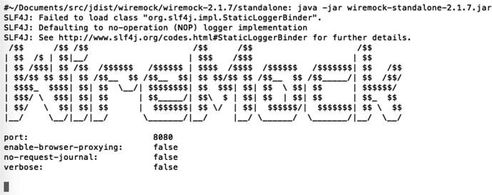
Figure 2-3.
Startup banner running the wiremock.org stub server with the java -jar option
Figure 2-4.
The json body of an HTTP POST used to configure wiremock to return a predetermined HTTP response
It is incredibly easy to launch Wiremock with a simple java -jar approach: Just execute java -jar wiremock.jar, and it starts right up listening for HTTP requests on port 8080 (which is configurable).
Once it is started, you can make HTTP/json calls to configure the request-response pairs to mimic your back-end
. You POST the json to http://<host>:<port>/__admin/mappings/new. Then you can save those calls in a SOAP UI, Chrome Postman, or JMeter script and execute them right before the load test. In Figure 2-4 json says, “If Wiremock receives a GET to /some/thing, then return ‘Hello world!’ as the response, but only after waiting 5 seconds.”
Once you have POSTed the preceding code to http://localhost:8080/__admin/mappings/new, you should try out the new stub as shown in Figure 2-5.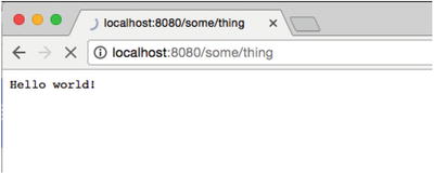
Figure 2-5.
Using Chrome to test the newly created wiremock configuration (Figure 2-4)
… and sure enough, the browser doesn’t paint “Hello world!” until Wiremock waits the 5000 milliseconds that we asked for using the fixedDelayMilliseconds attribute in the json.
That wasn’t too difficult, right? To summarize, download the Wiremock jar and run it as java -jar. Then submit Wiremock json-over-HTTP configuration messages to essentially teach Wiremock
which responses to return for each HTTP request supported by your back-end. Lastly, start your app and watch it submit requests to Wiremock, and Wiremock will return the responses that you configured. That’s it.
Local Load Generation
With the Code First approach in mind, the heart of the two-machine developer tuning environment (Figure 2-2) is your code—a single JVM for the web tier that makes calls to a single JVM for the application tier.
Here are the other parts we are concerned with.
First are the stub servers we just talked about. They replace the mainframe and the cloud services. Vetting the actual systems for performance will have to wait for later, probably in an integration testing environment.
Ultimately, some monitoring will be sprinkled in, but the last component to go into the developer tuning environment is the load generator, the topic of this section.
Quick Overview of Load Generation
A load generator is a network traffic generator. We use it to stress a network-enabled software application, like a SOA or the server-side portion of a web-application, to see if the responses are fast enough and to make sure it doesn’t crash.
Of course, it wouldn’t be helpful to sling random traffic at a web application—we’d need to submit the exact kind of web requests the web app was designed to process. For this purpose, most load generators, like JMeter, use a record-and-playback approach to get the traffic just right. It works like this: on an otherwise idle system, you manually traverse your application using a web browser while a special tool (which comes with a load generator) records the network requests made by your browser.
The output of that recording is a tool-specific script that can replay, verbatim, that single user’s traffic, thus stressing out the SUT a little bit. Then, to model a dynamic workload and move away from the verbatim recording, you enhance the script to log on a (data-driven) variety of users and operate on a (data-driven) variety of “things” in the SUT—whatever things the SUT deals in—shopping for kayaks, a dating service for manatees, delivering news stories, whatever. Hardware permitting, load generators can spin up as many threads as you like to simulate a larger number of users.
Load Generator Responsibilities
A load generator has these main responsibilities
:
- 1.To record network traffic as you traverse a system, and save the navigation details to a script.
- 2.To allow you to edit/debug/enhance the script, so that it more closely resembles a production load.
- 3.To run the script in a single thread, and to enable multiple threads to run the same script concurrently, thus applying load to your system. This is “load generation.”
- 4.To display the response time, throughput and other test results via live graphs/displays and/or via post-test reports.
The “Load Generator” in Figure 2-2 specifically refers to responsibility 3, load generation. You can take care of responsibilities 1, 2 and 4 wherever and however you need to.
In fact, the startup banner for the JMeter load generator addresses this very concern (Figure 2-6).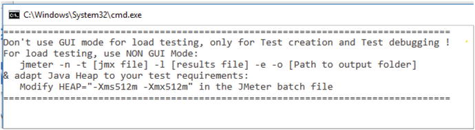
Figure 2-6.
Warning from JMeter not to use the GUI during a load test
The idea is to create, record, and refine your load script using JMeter GUI Mode. Running a small amount of load, perhaps less than ten requests per second is acceptable, too. Do all of this with the JMeter GUI Mode. But when it comes to running more than 10RPS, your safest best to avoiding performance problems in the load generator itself is by running JMeter in NON GUI Mode, aka from the command line, or headless. The JMeter startup banner in Figure 2-6 even shows how to do this. Here is an example:
- 1.First start the JMeter GUI and create your load plan and save it to myLoadPlan.jmx.
- 2.Copy the myLoadPlan.jmx file to your developer tuning environment, where JMeter needs to be installed.
- 3.Run this command:$JMETER_HOME/bin/jmeter -n -t myLoadPlan.jmx -l test001.jtl -e -o dirTest001where test001.jtl is a text data file in which JMeter will write results from the test and dirTest001 is a folder that JMeter will create and use to hold a performance report after the test finishes.
As long as RAM and CPU consumption
for the JMeter process stay relatively low, perhaps below 20% for both, then I have had no problems running JMeter on the same machine as the SUT. If you are still skeptical, see if performance dramatically improves by moving the load generation to another box on the same subnet.
CPU Consumption by PID
Having just a single person on a team care about performance is a tough, uphill battle. But when you have a few (or all) coworkers watching out for problems, making sure results are reported, researching performance solutions, and so on, then performance is much more manageable.
So to get (and keep) others on-board and interested, a certain amount of performance transparency is required to better keep others up-to-date. For example, everyone knows how to use top and TaskMgr to watch for CPU consumption. But did you watch it for the duration of the test, or did you take your eyes off it while looking at the flood of other metrics? We should all be good skeptics for each other when troubleshooting, and a basic CPU consumption graph for the duration of the test really helps answer these questions before they’re asked.
But the task of watching CPU is more work when you’re trying to watch it on multiple machines, or as well in our case, trying to distinguish which of the many processes on a single machine has high/spiky CPU. My point here is that it is worth the time to regularly create and share easy-to-understand graphs and metrics, and furthermore in the special case of CPU consumption, there is a void of open-source/free tools that will graph CPU consumption over time for individual process IDs (PIDs)
.
I would like to quickly highlight one of the few tools that can do this, and it just so happens that this tool not only works with JMeter, but its results can be displayed on the same graph as any other JMeter metrics. The tool is called PerfMon
and it comes from jmeter-plugins.org at
https://jmetr-plugins.org/wiki/PerfMon/
(see Figure 2-7).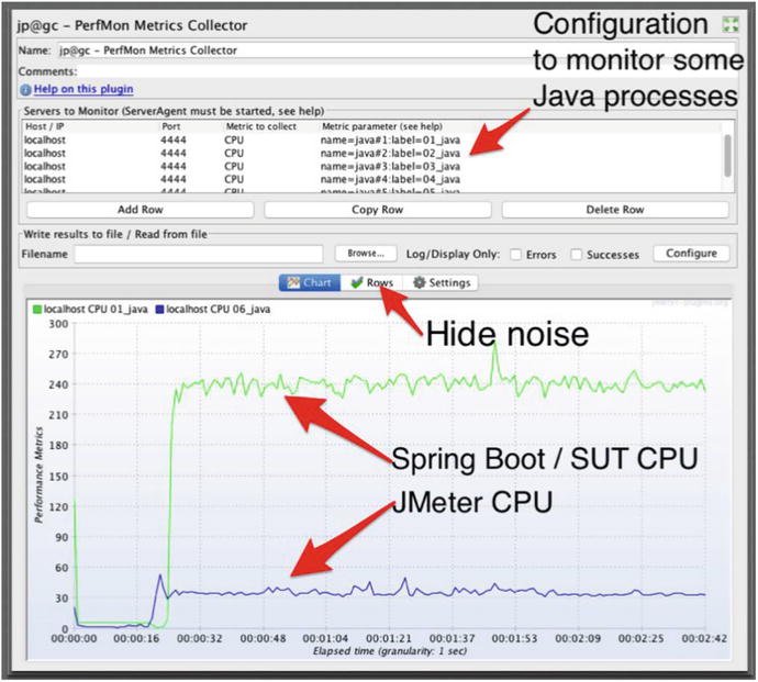
Figure 2-7.
. PerfMon from jmeter-plugins.org allows you to monitor CPU andmany other metrics
Here are a few notes:
- Because the i7 processor for this test has eight cores, if a single line reached 800, that would mean the system is 100% consumed. For six cores, 600 is the max. In this graph, we have two lines, 240 and 40. 240+40=280, and 280/800 = 35% CPU.
- In the pane at the top, I have configured PerfMon to capture CPU metrics for six different Java processes. Unfortunately, I had to use top on my MacBook to confirm which process was using ∼240 and which was ∼40.
- Sometimes there are many lines with low CPU consumption that get in the way. The “hide noise” label in Figure 2-3 shows one way to temporarily remove lines with very low consumption that make the graph noisy. Auto scaling, color selection, hiding lines, and other great graph refinement features are documented here:
I use these graphs mainly to confirm that CPU remains relatively low, perhaps below 20%, for the load generator and any stub servers. The JMeter line reads at about 40, so 40/800=5% CPU, which is less than 20%, so JMeter CPU consumption is sufficiently low.
PerfMon works on just about every platform available. Here are two other tools that also graph resource consumption by PID. Neither of them have native Windows support, although you could try to run them in a Linux/Docker container:
Regardless of the tool you use
, having PID-level metrics to show CPU and other resource consumption is critical understanding whether you have misbehaving processes in your modest tuning environment. When reporting on your results, remember to point out the portion of consumption that comes from test infrastructure—the load generator and the stub server(s).
Comparison Metrics
A few years ago, I ran a JMeter test
on a do-nothing Java servlet that was deployed to Tomcat and was on the same machine as JMeter. Had I seen 1,000 requests-per-second, I think I would have been impressed. But in my updated version of this test, I saw more than 2,800 requests per second with about 35% CPU consumption. And 99% of the requests completed in less than 1.3 ms (milliseconds), as measured at the servlet (by glowroot.org).
These results were so astoundingly good that I actually remember them. I can’t find my car keys, but I remember how much throughput my four-year-old laptop can crank out, and I recommend that you do the same. Why? These numbers are incredibly powerful, because they keep me from thinking that Java is inherently slow. They can also help with similar misunderstandings about whether Tomcat, JMeter, TCP or even my MacBook are inherently slow.
Lastly, these results (Figure 2-8) make me think that even on a single machine in this small developer tuning environment, there is a ton of progress that can be made.
Figure 2-8.
Response time and throughput metrics
for a do-nothing Java servlet. Metrics from Glowroot.org. Intel(R) Core(TM) i7-3615QM CPU @ 2.30GHz, Java 1.8.0_92-b14.
Don’t Forget
The environments in Figure 2-1 and Figure 2-2 are substantially different! This chapter has discussed all the things that were excluded from the design of the developer modest tuning environment (Figure 2-1). We are cutting scope so we can vet the performance of the part of the system that we developers are responsible for—the code. Hence the Code First mantra.
I can appreciate that the small developer tuning environment I’m proposing looks unconventional, so much so that you might wonder whether it reproduces realistic enough conditions to make tuning worthwhile. In short, the appearances of this environment design seem wildly artificial.
In response, I will say that this particular environment design addresses a longstanding specific strategic need that helps avoid last-minute rush-job performance tuning efforts that have left our systems, and perhaps even our industry, a bit unstable. The modest tuning environment also helps us identify and abandon poorly performing design approaches earlier in the SDLC.
Few question the efficacy of a wind tunnel to vet aerodynamics or a scale-model bridge to assess stability. The wind tunnel and the model bridge are wildly artificial, yet widely accepted test structures inserted into the development process to achieve strategic purposes. This small developer tuning environment design is our technology offering to address long standing, industry-wide performance issues.
There will be skeptics that say that a small environment can never provide a close enough approximation of a production workload. These are generally the same people that feel that performance problems are only rarely reproducible. To this group I would say that the modest tuning environment is a reference environment that we use to demonstrate how to make our systems perform. We won’t fix everything, but we have to begin to demonstrate our resilience somewhere and somehow.
What’s Next
In the Introduction, I talked about how performance defects thrive in Dark Environments. Well, not all environments are Dark. Sometimes there is an unending sea of metrics and it’s tough to know which to use to achieve performance goals. The next chapter breaks down metrics into a few high-level categories and talks about high to use each to achieve performance goals. There are also a few creative solutions to restructuring your load tests that can help avoid wandering around lost in a completely Dark Environment.
Footnotes
1
If you’d like more detail, there are more service virtualization tools. See
http://blog.trafficparrot.com/2015/05/service-virtualization-and-stubbing.html
And this book:
http://www.growing-object-oriented-software.com/
.