
2.6. FERRITE CONSTITUTIVE RELATIONS 39
H
0
H
0
sinθ
0
cosϕ
0
H
0
sinθ
0
sinϕ
0
H
0
cosθ
0
ϕ
0
θ
0
Z
X
Y
Figure 2.11: Illustration of an arbitrarily oriented DC biasing magnetic field.
Here, the case of
N
H
0
in the direction (
0
, '
0
) is taken from Tyras [
35]:
ΠD
2
6
4
C .
0
/ sin
2
0
cos
2
'
0
0
2
sin
2
0
sin 2'
0
C j k cos
0
0
2
sin
2
0
sin 2'
0
j k cos
0
C .
0
/ sin
2
0
sin
2
'
0
0
2
sin 2
0
cos '
0
C j k sin
0
sin '
0
0
2
sin 2
0
sin '
0
j k sin
0
cos '
0
0
2
sin 2
0
cos '
0
j k sin
0
sin '
0
0
2
sin 2
0
sin '
0
C j k sin
0
cos '
0
0
.
0
/ sin
2
0
3
7
5
: (2.27)
Note that there is a conjugate symmetry in the off-diagonal elements of the permeability
tensor of Eq. (2.27), e.g.,
ji
D
ij
for i; j D x; y; z. Also note that when dealing with the
permeability tensor, one should carefully handle the time-harmonic dependence, assumed to
be either e
Cj!t
, (which is more common), or e
j!t
, (as some authors do). In Eq. (2.27), a
dependence of e
Cj!t
is assumed. In those cases, in which the choice is e
j!t
, the sign of j k is
reversed.
2.6.6 PERMEABILITY TENSOR: TAKING LOSSES INTO ACCOUNT
Microwave ferrite losses are accounted for in magnetization equation in some of the alternative
formal treatments given in Eqs. (2.12), (2.13), and (2.16). It should be noted that a clear under-
standing of the loss mechanism is difficult to be achieved [12]. Another important observation
is that in the above equations, the additional loss term
N
M = or
N
M .d
N
M =dt/ is perpendicular
to
N
M
N
H . is represents energy storage, or equivalently, a space lag of 90
ı
. However, since
N
M rotates about its equilibrium orientation, this space lag of 90
ı
is equivalent to a time lag of a
quarter of the period [12]. is, in turn, yields a complex susceptibility tensor ŒX , whose real

40 2. TUNABLE MATERIALS–CHARACTERISTICS AND CONSTITUTIVE PARAMETERS
part represents energy storage and imaginary part denotes losses. Baden Fuller [12] has pre-
sented a solution of the magnetization Eq. (2.12). e solution states that for the lossy case,
expressions for susceptibility and permeability are similar to those in Eqs. (2.17) and (2.21). In
fact, it is provided that resonance frequency !
0
is substituted with a complex value
!
0
.
!
0
C j!˛
/
; (2.28)
where ˛ is the damping factor.
e above is exactly what should be expected from previous explanation about losses caus-
ing a quarter-period time lag. erefore, the permeability tensor is the same for any case given
in the previous sections, but
and
k
are [12],
D
0
C
0
M
s
.
0
H
0
C j
0
!˛
/
.
0
H
0
C j
0
!˛
/
2
!
2
D
0
1 C
!
m
.
!
0
C j˛!
/
.
!
0
C j˛!
/
2
!
2
(2.29)
k
D
0
M
s
!
.
0
H
0
C j
0
!˛
/
2
!
2
D
0
!
!
m
.
!
0
C j˛!
/
2
!
2
; (2.30)
where !
0
and !
m
are taken from Eq. (2.19) and the damping factor ˛ is estimated from the mea-
surements of microwave losses around the gyromagnetic resonance (! D !
0
). Detailed expres-
sions for the complex susceptibility tensor ŒX , when losses are included, are given in [12, 14]. A
graphic representation of the real and imaginary part of these complex susceptibilities is shown in
Figure 2.12. ese curves are obtained by varying either the frequency of the RF microwave sig-
nal (!) or the DC biasing magnetic field H
0
, which corresponds to a variation of !
0
D
0
H
0
.
However, it should always be ensured that the ferrite is operated at its saturated state, e.g.,
H
0
> 4M
S
.
e gyromagnetic resonance phenomenon occurs when the forced precession frequency
is equal to the Larmor free precession frequency !
0
, namely, ! D !
0
. When losses are not
accounted for, and k tend to infinity at ! D !
0
. In contrast, when losses are taken into account,
the permeabilities or the susceptibilities become maximum but remain finite at gyromagnetic
resonance, as is obvious from Eqs. (2.29) and (2.30), or from Figure 2.5. Note that:
j X
xy
D j
X
0
xy
j X
00
xy
D X
00
xy
C j X
0
xy
: (2.31)
e damping factor ˛ can be obtained from the imaginary part (representing losses) of
the susceptibility near resonance (which is usually measured) and is related to the so-called
“resonance linewidth H or !.”
As shown in Figure 2.13, the resonance linewidth is the width of the resonance curve
between the points where the magnitude of X
00
xx
(or X
00
xy
or k) becomes half its maximum value.
Under the approximation of small losses ˛ 1, (common for microwave ferrites), ˛
2
C 1 1
and the maximum values at resonance ! D !
0
are the following [12, 14]:
for ! D !
0
$ X
00
xx;max
D k
00
max
D
!
m
2˛ !
0
: (2.32)

2.6. FERRITE CONSTITUTIVE RELATIONS 41
?′
xx
?′′
xx
?′
xy
?′′
xy
0.5
1.51.0 2.0
1.50.5 1.0 2.0
1.50.5 1.0 2.0
1.5
0.5
1.0 2.0
(a)
(b)
ω
0
ω
ω
0
ω
ω
0
ω
ω
0
ω
Figure 2.12: Graphic representation of typical ferrite complex susceptibilities.
?′′
xx
?′′
max
?′′
max
ω
0
ω
2
H
0
( )
H
1
ΔH
H
r
H
2
0
Figure 2.13: Gyromagnetic resonance and definition of the resonance linewidth .H or !
0
/.
..................Content has been hidden....................
You can't read the all page of ebook, please click here login for view all page.