Chapter 5
The Basics of Electronic Engine Control
Chapter Outline
Motivation for Electronic Engine Control
Federal Government Test Procedures
Concept of an Electronic Engine Control System
Definition of Engine Performance Terms
Effect of Air/Fuel Ratio on Performance
Effect of Spark Timing on Performance
Effect of Exhaust Gas Recirculation on Performance
Electronic Fuel-Control System
Exhaust gas oxygen concentration
Frequency and deviation of the fuel controller
Analysis of Intake Manifold Pressure
Engine control in the vast majority of engines means regulating fuel and air intake as well as spark timing to achieve desired performance in the form of power output. Until the 1960s, control of the engine output torque and RPM was accomplished through some combination of mechanical, pneumatic, or hydraulic systems. Then, in the 1970s, electronic control systems were introduced.
This chapter is intended to explain, in general terms, the theory of electronic control of a gasoline-fueled, spark-ignited automotive engine. Chapter 7 explains practical digital control methods and systems. The examples used to explain the major developments and principles of electronic control have been culled from the techniques of various manufacturers and do not necessarily represent any single automobile manufacturer at the highest level of detail.
Motivation for Electronic Engine Control
The initial motivation for electronic engine control came in part from two government requirements. The first came about as a result of legislation to regulate automobile exhaust emissions under the authority of the Environmental Protection Agency (EPA). The second was a thrust to improve the national average fuel economy by government regulation. The issues involved in these regulations along with normal market forces continue to motivate improvements in reduction of regulated gases as well as fuel economy. Electronic engine control is only one of the automotive design factors involved in fuel economy improvements. However, this book is only concerned with the electronic systems.
Exhaust Emissions
Although diesel engines are in common use in heavy trucks, railroads, and some pick-up trucks, the gasoline-fueled engine is the most commonly used engine for passenger cars and light trucks in the United States. This engine is more precisely termed the gasoline-fueled, spark-ignited, four-stroke/cycle, normally aspirated, liquid-cooled internal combustion engine. It is this engine, which is denoted the SI engine, that is discussed in this book. The following discussion of exhaust emission regulations applies to the SI engine.
The engine exhaust consists of the products of combustion of air and gasoline mixture. Gasoline is a mixture of chemical compounds that are called hydrocarbons. This name is derived from the chemical formation of the various gasoline compounds, each of which is a chemical union of hydrogen (H) and carbon (C) in various proportions. Gasoline also contains natural impurities as well as chemicals added by the refiner. All of these can produce undesirable exhaust elements. The combustion of gasoline in an engine results in exhaust gases, including CO2, H2O, CO, oxides of nitrogen, and various hydrocarbons.
During the combustion process, the carbon and hydrogen combine with oxygen from the air, releasing heat energy and forming various chemical compounds. If the combustion were perfect, the exhaust gases would consist only of carbon dioxide (CO2) and water (H2O), neither of which is considered harmful to human health in the atmosphere. In fact, both are present in an animal’s breath.
Unfortunately, the combustion of the SI engine is not perfect. In addition to the CO2 and H2O, the exhaust contains amounts of carbon monoxide (CO), oxides of nitrogen (chemical unions of nitrogen and oxygen that are denoted NOx), unburned hydrocarbons (HC), oxides of sulfur, and other compounds. Some of the exhaust constituents are considered harmful and are now under the control of the federal government. The exhaust emissions controlled by government standards are CO, HC, and NOx.
Automotive exhaust emission control requirements began in the United States in 1966 when the California state regulations became effective. Since then, the federal government has imposed emission control limits for all states, and the standards became progressively tighter throughout the remainder of the twentieth century and will continue to tighten in the twenty-first century. Auto manufacturers found that the traditional engine controls could not control the engine sufficiently to meet these emission limits and maintain adequate engine performance at the same time, so they turned to electronic controls.
Fuel Economy
Everyone has some idea of what fuel economy means. It is related to the number of miles that can be driven for each gallon of gasoline consumed. It is referred to as miles per gallon (MPG) or simply mileage. In addition to improving emission control, another important feature of electronic engine control is its ability to improve fuel economy.
It is well recognized by layman and experts alike that the mileage of a vehicle is not unique. Mileage depends on the size, shape, and weight of the car as well as how the car is driven. The best mileage is achieved under steady cruise conditions. City driving, with many starts and stops, yields worse mileage than steady highway driving. In order to establish a regulatory framework for fuel economy standards, the federal government has established hypothetical driving cycles that are intended to represent how cars are operated on a sort of average basis.
The government fuel economy standards are not based on one car, but are stated in terms of the average rated miles per gallon fuel mileage for the production of all models by a manufacturer for any year. This latter requirement is known in the automotive industry by the acronym CAFE (corporate average fuel economy). It is a somewhat complex requirement and is based on measurements of the fuel used during a prescribed simulated standard driving cycle.
Federal Government Test Procedures
For an understanding of both emission and CAFE requirements, it is helpful to review the standard cycle and how the emission and fuel economy measurements are made. The U.S. federal government has published test procedures that include several steps. The first step is to place the automobile on a chassis dynamometer, like the one shown in Figure 5.1.

Figure 5.1 Chassis dynamometer.
A chassis dynamometer is a test stand that holds a vehicle such as a car or truck. It is equipped with instruments capable of measuring the power that is delivered at the drive wheels of the vehicle under various conditions. The vehicle is held on the dynamometer so that it cannot move when power is applied to the drive wheels. The drive wheels are in contact with two large rollers. One roller is mechanically coupled to an electric generator that can vary the load on its electrical output. The other roller has instruments to measure and record the vehicle speed. The generator absorbs and provides a measurement of all mechanical power that is delivered at the drive wheels to the dynamometer. The power is calculated from the electrical output in the correct units of kW or Hp (horsepower where 1 Hp = 0.746 kW). The controls of the dynamometer can be set to simulate the correct load (including the effects of tire rolling resistance and aerodynamic drag) and inertia of the vehicle moving along a road under various conditions. The conditions are the same as if the vehicle actually were being driven except for wind loads.
The vehicle is operated according to a prescribed schedule of speed and load to simulate the specified trip. One driving cycle simulates an urban trip and another simulates a highway trip. Over the years, the hypothetical driving cycles for urban and rural trips have evolved. Figure 5.2 illustrates sample driving cycle trips (one for each) that demonstrate the differences in those hypothetical test trips. It can be seen that the urban cycle trip involves acceleration, deceleration, stops, starts, and steady cruise such as would be encountered in a “typical” city automobile trip of 7.45 miles (12 km). The highway schedule takes 765 seconds and simulates 10.24 miles (16.5 km) of highway driving.
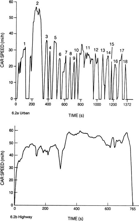
Figure 5.2 Federal driving schedules (Title 40 United States Code of Federal Regulations).
During the operation of the vehicle in the tests, the exhaust is continuously collected and sampled. At the end of the test, the absolute mass of each of the regulated exhaust gases is determined. The regulations are stated in terms of the total mass of each exhaust gas divided by the total distance of the simulated trip.
Fuel Economy Requirements
In addition to emission measurement, each manufacturer must determine the fuel consumption in MPG for each type of vehicle and must compute the corporate average fuel economy (CAFE) for all vehicles of all types produced in a year. Fuel consumption is measured during both an urban and a highway test, and the composite fuel economy is calculated.
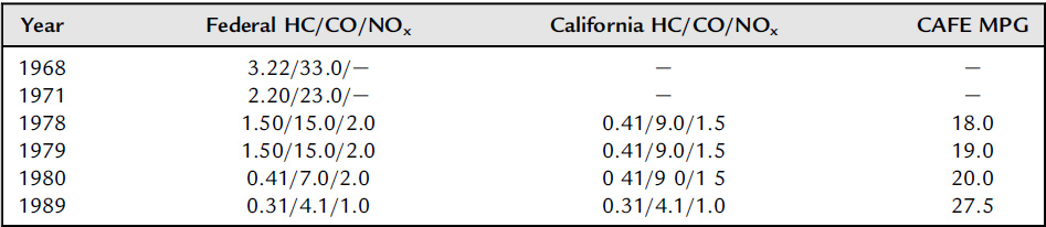
Table 5.1 is a summary of the exhaust emission requirements and CAFE standards for a few representative years. It shows the emission requirements and increased fuel economy required, demonstrating that these regulations have become and will continue to become more stringent with passing time. Not shown in Table 5.1 is a separate regulation on nonmethane hydrocarbon (NMHC). Because of these requirements, each manufacturer has a strong incentive to minimize exhaust emissions and maximize fuel economy for each vehicle produced.
Table 5.1 Emission and MPG requirements.
New regulations for emissions have continued to evolve and encompass more and more vehicle classes. Present-day regulations affect not only passenger cars but also light utility vehicles and both heavy- and light-duty trucks. Furthermore, regulations apply to a variety of fuels, including gasoline, diesel, natural gas, and alcohol-based fuels involving mixtures of gasoline with methanol or ethanol.
As an example, we present below the standards that were written for the vehicle half-life (5 years or 50,000 miles–whichever comes first) and full life cycle (10 years or 100,000 miles) as of 1990. The standards are:
| HC | 0.31 g/mi |
| CO | 4.20 g/mi |
| NOx | 0.60 g/mi (non-diesel) |
| 1.25 g/mi (diesel) |
These regulations were phased in according to the following schedules:
Model year 1994: 40%
Model year 1995: 80%
Model year 1996: 100%
There are many details to these regulations that are not relevant to the present discussion. However, the regulations themselves are important in that they provided motivation for expanded electronic controls.
Meeting the Requirements
Unfortunately, as seen later in this chapter, meeting the government regulations causes some sacrifice in performance. Moreover, attempts to meet the standards exemplified by Table 5.1 using mechanical, electromechanical, hydraulic, or pneumatic controls like those used in pre-emission control vehicles have not been cost-effective. In addition, such controls cannot operate with sufficient accuracy across a range of production vehicles, over all operating conditions, and over the life of the vehicle to stay within the tolerance required by the EPA regulations. Each automaker must verify that each model produced will still meet emission requirements after traveling 100,000 miles. As in any physical system, the parameters of automotive engines and associated peripheral control devices can change with time. An electronic control system has the ability to automatically compensate for such changes and to adapt to any new set of operating conditions and make electronic controls a desirable option in the early stages of emission control.
The Role of Electronics
The use of digital electronic control has enabled automakers to meet the government regulations by controlling the system accurately with excellent tolerance. In addition, the system has long-term calibration stability. As an added advantage, this type of system is very flexible. Because it uses microcomputers, it can be modified through programming changes to meet a variety of different vehicle/engine combinations. Critical quantities that describe an engine can be changed relatively easily by changing data stored in the system’s computer memory.
Additional cost incentive
Besides providing control accuracy and stability, there is a cost incentive to use digital electronic control. The system components—the multifunction digital integrated circuits—are decreasing in cost, thus decreasing the system cost. From about 1970 on, considerable investment was made by the semiconductor industry for the development of low cost, multifunction integrated circuits. In particular, the microprocessor and microcomputer have reached an advanced state of capability at relatively low cost. This has made the electronic digital control system for the engine, as well as other on-board automobile electronic systems, commercially feasible. As pointed out in Chapter 3, as multifunction digital integrated circuits continue to be designed with more and more functional capability through very large scale integrated circuits (VLSI), the costs continue to decrease. At the same time, these circuits offer improved electronic system performance in the automobile.
In summary, the electronic engine control system duplicates the function of conventional legacy fluidic control systems, but with greater precision and long-term stability via adaptive control processes. It can optimize engine performance while meeting the exhaust emission and fuel economy regulations and can adapt to changes in the plant.
Concept of an Electronic Engine Control System
In order to understand electronic engine control, it is necessary to understand some fundamentals of how the power produced by the engine is controlled. Any driver understands intuitively that the throttle directly regulates the power produced by the engine at any operating condition. It does this by controlling the airflow into the engine.
In essence the engine is an air pump such that at any RPM, the mass flow rate of air into the engine varies directly with throttle plate angular position (see Figure 5.3).
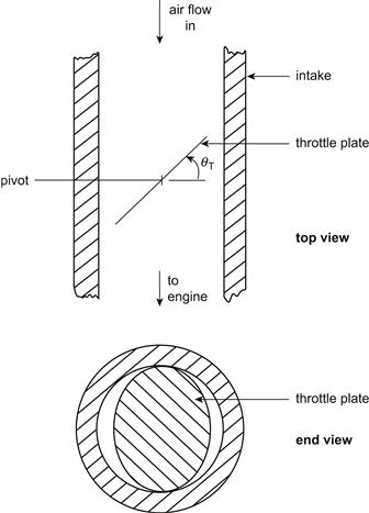
Figure 5.3 Intake system with throttle plate.
As the driver depresses the accelerator pedal, the throttle angle (θT in Figure 5.3) increases, which increases the cross-sectional area through which the air flows, reducing the resistance to airflow and thereby allowing an increased airflow into the engine. A model for the airflow vs. throttle angle and engine RPM is given later in this chapter. The role of fuel control is to regulate the fuel that is mixed with the air so that it increases in proportion to the airflow. As we will see later in this chapter, the performance of the engine is affected strongly by the mixture (i.e., by the ratio of air to fuel). However, for any given mixture the power produced by the engine is directly proportional to the mass flow rate of air into the engine. In the U.S. system of units as a rough “rule of thumb,” an airflow rate of about 6 lb/h produces 1 horsepower of usable mechanical power at the output of the engine. Metric units have come to be more commonly used, in which engine power is given in kilowatts (kW) and air mass is given in kilograms (kg). Denoting the power from the engine Pb, the linear model for engine power is given by
![]()
where Pb is the power from the engine (hp or kW), ![]() the mass airflow rate (kg/sec) or (slugs/sec), and K the constant relating power to airflow (kW/kg/sec) or (hp/lb/sec). Of course, it is assumed that all parts of the engine, including ignition timing, are functioning correctly for this relationship to be valid.
the mass airflow rate (kg/sec) or (slugs/sec), and K the constant relating power to airflow (kW/kg/sec) or (hp/lb/sec). Of course, it is assumed that all parts of the engine, including ignition timing, are functioning correctly for this relationship to be valid.
We consider next an electronic engine control system that regulates fuel flow to the engine. An electronic engine control system is an assembly of electronic and electromechanical components that continuously varies the fuel and spark settings in order to satisfy government exhaust emission and fuel economy regulations. Figure 5.4 is a block diagram (at the most abstract level) of a generalized electronic engine control system.
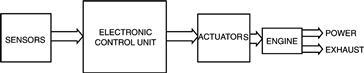
Figure 5.4 Generic electronic engine control system.
It will be explained later in this chapter that an automotive engine control has both open-loop and closed-loop operating modes (see Chapter 1). As explained in Chapter 1, a closed-loop control system requires measurements of certain output variables such that the controller can calculate the state of the system being controlled, whereas an open-loop system does not. The electronic engine control system receives input electrical signals from the various sensors that measure the state of the engine. From these signals, the controller generates output electrical signals to the actuators that determine the correct fuel delivery and spark timing.
Models for and performance analysis of automotive engine control system sensors and actuators are discussed in Chapter 6. As mentioned, the configuration and control for an automotive engine control system are determined in part by the set of sensors that is available to measure the variables. In many cases, the sensors available for automotive use involve compromises between performance and cost. In other cases, only indirect measurements of certain variables are feasible. From measurement of these variables, the desired variable is found by computation.
Figure 5.5 is a form of overall engine electronic control at a very abstract level. There is a fuel-metering system to set the air–fuel mixture flowing into the engine through the intake manifold. Spark control determines when the air–fuel mixture is ignited after it is compressed in the cylinders of the engine. The power is delivered at the driveshaft and the gases that result from combustion flow out from the exhaust system. In the exhaust system, there is a valve to control the amount of exhaust gas being re-circulated back to the input, and a catalytic converter to further control emissions. The addition of re-circulated exhaust gas to the engine intake, as well as various sensors and actuators depicted in Figure 5.5, is explained later in this chapter. In addition, there is a subsystem that collects the evaporating fuel vapors in the fuel tank to prevent them from being vented to the atmosphere. These fuel vapors are later sent to the intake system as a small component of fuel being supplied to the engine. This subsystem is denoted EVAP in Figure 5.5.
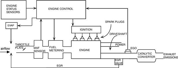
Figure 5.5 Engine functions and control diagram.
At one stage of development, the electronic engine control consisted of separate subsystems for fuel control, spark control, and exhaust gas recirculation. The ignition system in Figure 5.5 is shown as a separate control system, although engine control is evolving toward an integrated digital system (see Chapter 7).
Inputs to Controller
Figure 5.6 identifies the major physical quantities that are sensed and provided to the electronic controller as inputs. They are as follows:
1. Throttle position sensor (TPS)
3. Engine temperature (coolant temperature) (CT)
4. Engine speed (RPM) and angular position
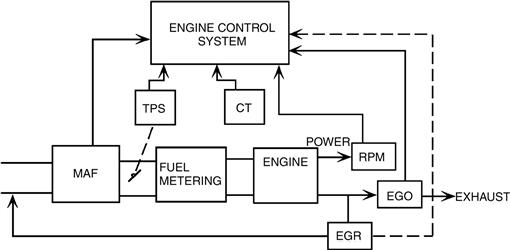
Figure 5.6 Major controller inputs from engine.
Output from Controller
Figure 5.7 identifies the major physical quantities that are outputs from the controller. These outputs are

Figure 5.7 Major controller outputs to engine.
This chapter discusses the various electronic engine control functions separately and explains how each function is implemented by a separate control system. Chapter 7 shows how these separate control systems are being integrated into one system and are implemented with digital electronics.
For certain readers of this book, a brief review of engine configuration and operation may be helpful. Although several types of engines have found application as the prime mover in automobiles, the one most commonly used continues to be the multicylinder, four-stroke IC engine as explained earlier in the chapter. The configuration and operation of electric propulsion (e.g., in hybrid vehicle) are discussed in Chapter 6.
The configuration of a single cylinder of an IC engine is depicted in Figure 5.8a. Mechanical power is produced by the engine in the form of torque acting on the rotating crank shaft. There are four basic engine processes that occur during the two complete revolutions of the crankshaft that occur during any single cycle of operation. This engine configuration includes a component called the piston, which fits within a cylinder and is mechanically linked to the crankshaft by the connecting rod. Airflow into and out of the cylinder is controlled by poppet valves (simply called the valves here). One of these is termed the intake valve and the other the exhaust valve. Additional components of the engine include a so-called “intake port system” consisting of a system of passageways (e.g., tubes) that direct fuel/air mixture into the engine and a so-called “exhaust port system” that directs the products of combustion out of the engine.
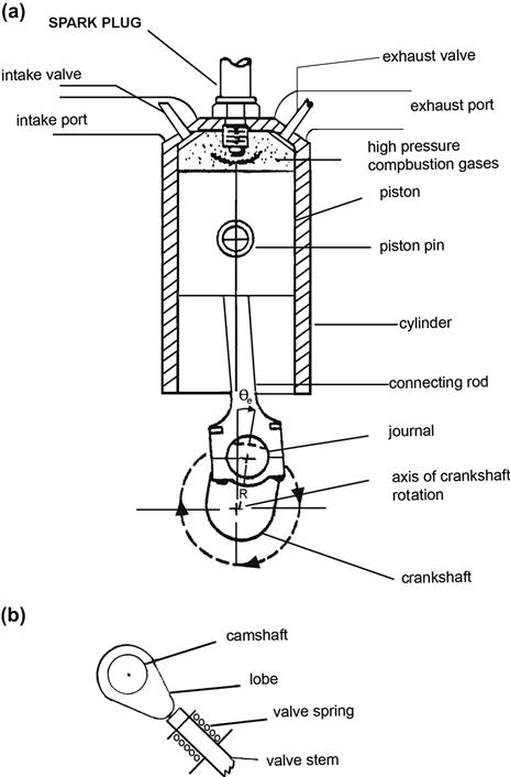
Figure 5.8 IC engine cylinder and cam actuation mechanism
During any single cycle of engine operation (involving two complete rotations of the crankshaft), there are four portions of the crankshaft rotation called strokes. Each stroke corresponds to piston (reciprocating) motion from its highest point (called “top-dead-center” or TDC) to the lowest point (called “bottom-dead-center” or BDC). These four strokes of any given engine cycle are termed intake, compression, power, and exhaust strokes. During the intake stroke, the piston moves from TDC to BDC. During most of this stroke, the intake valve is open and the exhaust valve is closed. During this stroke, air mixed with fuel is pumped into the cylinder by the positive differential pressure between the intake port and the cylinder internal pressure. During the compression stroke, the piston moves from BDC to TDC. Both intake and exhaust valves are closed. For an ideal IC engine, this compression is adiabatic and modeled by the following expression:
![]() (1)
(1)
where Vc is the cylinder contained volume (between the piston upper surface and the top of the combustion chamber), pc the combustion chamber pressure, and γ the ratio of specific heat at constant pressure to the specific heat at constant volume. For the intake air/fuel mixture ![]() for air/gasoline mixture.
for air/gasoline mixture.
The term adiabatic refers to a process with zero heat loss. The compression process for an actual engine is not adiabatic since heat is lost (e.g., through the cylinder sidewalls). The actual function pc(Vc) for a practical engine is shown graphically later in this chapter.
The difference between combustion chamber maximum volume (piston at BDC) and its minimum volume (at TDC) (which is often called the “clearance volume”) is called the cylinder displacement VD. The ratio of cylinder pressure at TDC to that at BDC is called the compression ratio r. At some point before the piston reaches TDC, the spark is generated and combustion of the fuel/air mixture is initiated and cylinder pressure rises rapidly.
During the next stroke, the power stroke, the cylinder pressure, acting on the piston via the connecting rod, applies a torque to the crankshaft. This expansion ideally would be adiabatic, but in fact is not adiabatic due to heat losses (as is demonstrated later from measurements made on an actual engine).
During the final stroke, the exhaust stroke, the piston again moves from BDC to TDC. The exhaust valve is open during most of this stroke, and the products of combustion (mostly CO2 and H2O) are pumped out of the cylinder into the exhaust system and released through this system to the atmosphere.
The actual point in the 720° crankshaft rotation angle at which the valves open and close (called valve timing) is determined by a mechanism that includes the camshaft and mechanical linkage connecting it to the valves. The camshaft, which is illustrated in Figure 5.8b, has lobes that force the valves open against the restoring forces of valve springs that otherwise hold the valves closed. The reader should imagine that the valves depicted in Figure 5.8a extend to the end of the valve stem depicted in Figure 5.8b. The camshaft is coupled via a gear system to the crankshaft such that it rotates at half the speed of the latter. This mechanism assures that the valves operate synchronously within each engine cycle. During the development period of any new engine design, the optimal valve timing is determined. In Chapter 6, the drive mechanism for the camshaft and the means for rotating it at half the crankshaft angular speed are explained with respect to a system known as variable valve phasing. For the present, however, the discussion is focused on basic engine processes.
Energy is produced by a four-stroke/cycle internal combustion engine only during the power stroke. The energy produced during this stroke must be greater than the energy required for the other strokes as well as by internal friction losses. Normally, in any well-designed engine the power stroke energy far exceeds the magnitude of all mechanical losses, thereby yielding net output energy.
A basic method of evaluating the output mechanical energy involves the so-called indicator diagram, which is also a plot of the pc vs. Vc for the entire cycle. Figure 5.9 represents an indicator diagram for an ideal engine cycle (in the sense of no heat loss to the engine) by the dashed curve and the pc(Vc) plot for an actual engine by the solid curve.
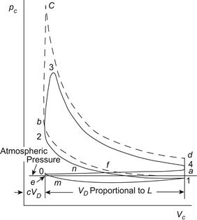
Figure 5.9 Indicator diagram for a four-stroke engine.
For the ideal engine cycle, the valves are assumed to open or close at exactly TDC or BDC. Any time delays associated with the gas dynamics of intake and exhaust are taken to be negligible. In Figure 5.9, point a is at BDC with the cylinder filled with fuel/air mixture. The segment from point a to point b corresponds to the compression stroke. Ignition occurs at point b and the combustion chamber pressure increases instantaneously to point c, which is the beginning of the power stroke. The power stroke is represented by the segment from point c to point d. At point d, the exhaust valve opens and pressure drops to the exhaust system pressure (pe) at point a. The segment from point a to point e corresponds to the exhaust stroke. At point e, the exhaust valve closes and the intake valve opens. The intake stroke corresponds to the segment from point e to point a where the cycle began and where the next engine cycle commences. For this ideal engine cycle, both intake and exhaust gas pressures are taken to be at atmospheric pressure.
The indicator diagram for an actual engine is depicted by the solid curve for which the compression stroke is the segment of the solid curve from point 1 to point 2. Notice that the pressure at point 1 is slightly below atmosphere pressure, which occurs because of pressure losses in the intake system. At point 2, ignition occurs and the pressure rises to its maximum value at point 3. The expansion from point 3 to point 4 is somewhat different in shape than the ideal adiabatic expansion due to heat losses. Pressure continues to drop after the exhaust valve opens (near point 4), but remains slightly above atmospheric pressure due to “back pressure” in the exhaust system. The exhaust stroke occurs between point 4 and point 0. The intake stroke occurs from point 0 to point 1 at pressure somewhat below atmospheric due to pressure drop across the throttle plate as well as some pressure losses in the intake system. From point 1, the cycle begins again.
The net energy/cycle (called the indicated energy, Wi) is given by the contour integral around the curve from points 1–6 below:
![]() (2)
(2)
The only positive contribution to this integral comes from the portion from point 3 to point 4 (i.e., the power stroke). The energy/cycle is influenced markedly by the timing of the valve openings and closing as will be explained in Chapter 7. As clearly shown from Figure 5.9, in any practical engine the indicator diagram deviates from the ideal as indicated by the continuous curve of Figure 5.9.
Definition of Engine Performance Terms
Several common terms are used to describe an engine’s performance, including the torque and power at various places in the engine and powertrain as well as cylinder pressure, crankshaft angular speed, fuel consumption and various combinations of these as explained below. It is these performance variables that are influenced by the electronic engine control. For an understanding of this controller influence, it is necessary to have the quantitative models for these performance variables as presented below.
Torque
Engine torque is produced on the crankshaft by the cylinder pressure pushing on the piston during the power stroke. In an IC, engine torque is produced at the crankshaft as explained below. The torque that is applied to the crankshaft is called “indicated torque Ti.” The output torque from the engine at the transmission end of the crankshaft differs from Ti due to friction and pumping losses and is called the brake torque (denoted Tb).
For an understanding of the various torques at different points in the powertrain, it is helpful to refer to Figure 5.10, which illustrates the geometry of a single cylinder in a four-stroke IC engine. Figure 5.10 shows the centerline of the cylinder which is a line along the cylinder axis through the crankshaft rotational center. The piston is connected via the connecting rod to the crankshaft. The connecting rod is fastened to the piston via the piston pin about which this rod can rotate. During the power stroke, a torque is applied to the crankshaft resulting from the force acting on the piston due to combustion chamber pressure acting through a lever arm which is proportional to the crank throw R and which varies with crankshaft angular position (θe). This torque is known as the indicated torque to distinguish it from other torque acting on the crankshaft and can be computed as explained below.
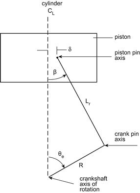
Figure 5.10 Schematic illustration of cylinder geometry.
Figure 5.10 presents the geometry of the piston, connecting rod, and crankshaft in a way which permits a model for the indicated torque Ti(θe) as a function of crankshaft angle (θe) to be developed. In Figure 5.10 the connecting rod length is denoted Lr and the radius from the crankshaft axis of rotation to the center of the connecting rod journal is denoted R. It is this radius of the crankshaft rotation which provides the lever arm for the production of indicated torque due to the force on the top of the piston due to combustion chamber pressure (Pc(θe)). In many engines, the piston pin is located slightly off the cylinder centerline (CL) in a plane that is orthogonal to the crankshaft axes of rotation, which benefits torque production. The piston pin offset from the cylinder CL is denoted δ in Figure 5.10. The angle between the connecting rod plane of symmetry and the cylinder axis is denoted β. Owing to the piston offset, the indicated torque for a piston on the down stroke is given by
![]() (3)
(3)
On the up stroke Ti is given by
![]() (4)
(4)
where A is the piston cross-sectional area. The factors ![]() represent the lever arm through which torque is applied to the crankshaft.
represent the lever arm through which torque is applied to the crankshaft.
The combustion chamber pressure for a representative four-stroke reciprocating IC engine is shown in Figure 5.11 for a complete engine cycle (720° of crankshaft rotation) beginning at –180° (BDC) for the start of compression and ending at 540° (BDC) at the end of intake stroke. Note that following ignition (point x), the pressure rises abruptly due to combustion reaching a maximum at a point (y) slightly beyond TDC.
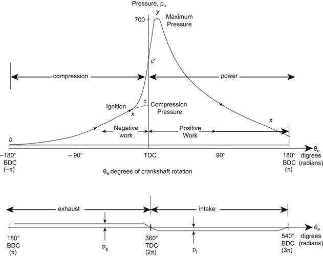
Figure 5.11 Exemplary plot of pc(θe).
The region of positive work for each cycle is indicated in the drawing as the power stroke (i.e., 0 to 180°). The fluctuations in combustion chamber pressure along with the geometry factor relating pc to Ti cause Ti to fluctuate with crankshaft angle and of course with time. However when the engine produces power, the time-average value for Ti (i.e., ![]() ) is positive:
) is positive:
![]()
There are other contributors to the total dynamic indicated torque at the crankshaft, including torques due to the reciprocating forces of the piston and connecting rod. The details of the reciprocating torque (Tr) are beyond the scope of this book and are not relevant to the present discussion, but in general increase quadratically with rotational speed. In addition, there are contributors to the torque at the crankshaft due to internal friction of the rotating and reciprocating components as well as due to pumping of intake and exhaust gases.
The indicated torque is the maximum available torque which is applied at each crankshaft segment for the corresponding cylinder. Typically, between each crankshaft “throw” are sleeve bearings that have friction. In addition to friction, there are negative torques applied to the crankshaft owing to the nonzero cylinder pressures—pe during exhaust and pi during intake – and a relatively large negative torque associated with compression. The time-average torque averaged over an engine cycle at the crankshaft output end is called the brake torque ![]() and is given by
and is given by
![]() (5)
(5)
where ![]() is the average torques associated with friction and pumping losses. It is this brake torque acting through the drivetrain that provides the torque to drive the vehicle. The drivetrain includes the transmission and other gear systems (e.g., differential) as explained in Chapter 7.
is the average torques associated with friction and pumping losses. It is this brake torque acting through the drivetrain that provides the torque to drive the vehicle. The drivetrain includes the transmission and other gear systems (e.g., differential) as explained in Chapter 7.
Power
One of the most important metrics for engine performance is output power. This power is related to the indicated torque applied to the crankshaft (as explained above). The instantaneous power applied to the crankshaft by the indicated torque is known as the indicated power (Pi[θe(t)]), given by
![]()
where
![]() (6)
(6)
The units for Pi(t) are Nm/sec (metric) or ft lb/sec (English units). Normally it is the average indicated power averaged over N engine cycles ![]() that is useful as a metric for engine available power (with θe in radians) is given by:
that is useful as a metric for engine available power (with θe in radians) is given by:
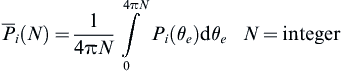 (7)
(7)
The appropriate unit for Pi is kW, although in the USA the popular unit (with the driving public) remains horsepower (Hp), where 1Hp = 0.75 kW and 550 ft lb/s.
The engine output power at the crankshaft is known as the brake power (Pb) since historically engine power was measured using a Prony brake. This brake power (in kW or Hp) is the difference between indicated power and the power associated with internal power losses due, e.g., to friction and pumping of the intake mixture and exhaust gases. Generally, the cycle-averaged friction and pumping power are combined and denoted ![]() . The brake power Pb is given by
. The brake power Pb is given by
![]() (8)
(8)
Measurements are readily made of Pfp by driving the engine from an external power source such as an electric dynamometer. The latter is an instrumented electric motor/generator having the capacity to absorb all brake power produced by the running engine under test. Normally, instrumentation permits measurements to be made of output torque, angular speed ωe, and Pb. It is also common practice to evaluate engine performance via the averaged torque at the engine output, which is called “brake torque” and is denoted Tb and which is related to Pb by the expression
![]() (9)
(9)
Another metric of performance for an engine is the so-called mean-effective pressure (mep). It is defined as the indicated work done on the piston (Wi) (given in Eqn (2)) divided by displacement volume VD. As in the case of torques, it is convenient to consider the indicated mep (imep) which is defined as
![]() (10)
(10)
where VD = V1 − V2 is the displacement, V1 the cylinder maximum volume (at BDC), and V2 the cylinder minimum volume at TDC; (i.e., clearance volume).
The imep (which has the dimensions of pressure) is the value of constant pressure, which, if acting during an engine cycle, would produce the work done on the crankshaft. There is also a friction mep (fmep):
![]() (11)
(11)
where Wf is the work done by the friction torque. The most commonly used mep is the brake mep (bmep), which is defined as
![]()
It has the units of pressure (e.g., N/m2 or lb/in2) and is the value of constant pressure acting over a full engine cycle to produce the output mechanical work/cycle.
Fuel Consumption
Fuel economy can be measured while the engine delivers power to the dynamometer. The engine is typically operated at a fixed RPM and a fixed brake power (fixed dynamometer load), and the fuel flow rate (in kg/hr or lb/hr) is measured. The fuel consumption is then given as the ratio of the fuel flow rate ![]() to the brake power output (Pb). This fuel consumption is known as the brake-specific fuel consumption, or BSFC. BSFC is a measurement of the fuel economy of the engine alone and is given by
to the brake power output (Pb). This fuel consumption is known as the brake-specific fuel consumption, or BSFC. BSFC is a measurement of the fuel economy of the engine alone and is given by
 (12)
(12)
The unit for BSFC is kg/(kW·hr) or (lb/CHp·hr) in British units. By improving the BSFC of the engine, the fuel economy of the vehicle in which it is installed is also improved. It is shown later in this chapter that electronic controls can optimize BSFC.
In gasoline-fueled engines, airflow into the engine at any operating angular speed (RPM) is determined by the throttle angular position. In fact, the throttle is the control by the driver that determines the engine output power.
As explained above, any internal combustion must pump air/fuel into its combustion chamber. If an IC engine were a perfect air pump, then at wide open throttle the air volume pumped into the engine for each complete engine cycle (i.e., two complete revolutions) would be its displacement volume Vd:
![]() (13)
(13)
where Ap is the piston cross-sectional area and Sc the cylinder stroke which is the distance traveled by the piston from TDC to BDC.
Formally, the volumetric efficiency ![]() is defined as the ratio of the mass of fresh mixture (i.e., air and fuel) that is actually pumped into the cylinder during an intake stroke at inlet air density to the mass of this mixture, which would fill the cylinder at the inlet air density. The volumetric efficiency for any given engine is determined empirically and varies with throttle angle, RPM, inlet pressure and temperature as well as exhaust pressure (pe). Assuming initially that all cylinders receive mixture at identical density the definition of
is defined as the ratio of the mass of fresh mixture (i.e., air and fuel) that is actually pumped into the cylinder during an intake stroke at inlet air density to the mass of this mixture, which would fill the cylinder at the inlet air density. The volumetric efficiency for any given engine is determined empirically and varies with throttle angle, RPM, inlet pressure and temperature as well as exhaust pressure (pe). Assuming initially that all cylinders receive mixture at identical density the definition of ![]() can be expressed by
can be expressed by
 (14)
(14)
where ![]() is the air intake mixture mass flow rate (slugs/sec) (or kg/sec), N the number of revolutions/sec, and ρi the inlet mixture density (slugs/ft3) (or kg/m3).
is the air intake mixture mass flow rate (slugs/sec) (or kg/sec), N the number of revolutions/sec, and ρi the inlet mixture density (slugs/ft3) (or kg/m3).
The variable ρi is the density of the mixture in the intake system downstream from the throttle plate in or near a cylinder inlet port. When inlet air density is defined at this point in the intake system, it provides a measurement of the air pumping efficiency of the cylinder and valves alone. It is this definition which is used for the present discussion. However, it should be noted that volumetric efficiency could be based on the air density at the input to the intake system (i.e., upstream of the throttle plate). With air density taken at this point, the volumetric efficiency is termed the overall volumetric efficiency. Unfortunately, it is not always convenient to measure the density of the inlet mixture which consists of air, fuel, and atmospheric water vapor. On the other hand, since fuel, airflow, and water vapor occupy the same volume and have the same intake volume flow rate ![]() , the following relationship is valid:
, the following relationship is valid:
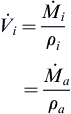 (15)
(15)
where ![]() is the mass flow rate of dry air and ρa the inlet density of dry air.
is the mass flow rate of dry air and ρa the inlet density of dry air.
For mixtures of air, water vapor, and gaseous or evaporated fuel, Dalton’s law of partial pressures states:
![]() (16)
(16)
where pi is the total inlet pressure, pa the partial pressure of air, pf the partial pressure of fuel, and pw the partial pressure of water vapor.
Each constituent (denoted k) of the inlet air mixture behaves as a perfect gas such that
![]() (17)
(17)
where R is the perfect gas law constant. Also, it can be shown that
 (18)
(18)
where Mk= mass of constituent k and mk = molecular mass of constituent k:
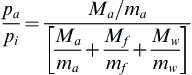
The air density in the mixture ρa is given by
![]() (19)
(19)
where ![]() is the fuel/air mass ratio, h the ratio of mass water vapor to the mass of air, ma = 29, and mw = 18.
is the fuel/air mass ratio, h the ratio of mass water vapor to the mass of air, ma = 29, and mw = 18.
In this form it is possible to compute inlet air density from measurements of total inlet air pressure (pi) and inlet absolute air temperature Ti as well as standard environmental variable measurements (e.g., relative humidity). As presently shown, Fi is determined by the fuel-control system to achieve certain engine performance requirements.
As explained earlier in this chapter, the engine power is regulated by the driver via an air valve in the form of a movable throttle plate in the intake system. Linkage connects the accelerator pedal to the throttle plate such that it partially restricts airflow into the engine. Typically, the throttle plate is in the form of a circular disk that pivots about a diametric axis in a cylindrical portion of the intake manifold (e.g., see Figure 5.3). Effectively, the airflow into the engine at any given engine angular speed (RPM) varies in proportion to the opening of this plate as represented by the throttle angle θT. This empirically determined volumetric efficiency is a convenient variable that can be used to characterize engine pumping efficiency during the development of a new engine control system and can also be used in fuel control of a production engine as explained later.
Engine Overall Efficiency
There are numerous ways to characterize the performance of an engine as indicated above. One of the most meaningful of these is the efficiency with which the engine converts the energy available in the fuel (in chemical form) to mechanical work. This efficiency, which we denote ηm, can be evaluated on an engine cycle by engine cycle basis. However, it is more convenient to express ηm as the ratio of the instantaneous mechanical power delivered to the load to the rate of change of available energy in the fuel being delivered:
![]()
where Pm is the mechanical power delivered to load (kW), ![]() the instantaneous mass flow rate of fuel (kg/sec), and Qf the energy content of fuel (joule/kg).
the instantaneous mass flow rate of fuel (kg/sec), and Qf the energy content of fuel (joule/kg).
Calibration
The definition of engine calibration is the setting of the air/fuel ratio and ignition timing for the engine for any given operating condition. With the new electronic control systems, calibration is determined by the electronic engine control system.
As will be shown later in this chapter, electronic engine control systems are based upon microprocessors or microcontrollers. Under program control, the engine control system determines the correct fuel delivery amount and the ignition timing as a function of driver command (via throttle setting) and other operating variables and parameters. Typically, these correct values are found from a table look-up process with interpolation. The calibration tables for any given engine configuration are found empirically as described below. As will also be shown below, an additional component of fuel delivery is determined from a closed-loop portion of the control.
The majority of present-day engines deliver fuel by means of an individual fuel injector associated with each cylinder. A fuel injector is essentially an electromechanical valve to which fuel, under pressure, is supplied. Chapter 6 explains the configuration and operation of fuel injectors. As will be explained later, each fuel injector delivers fuel in a pulse mode in which fuel quantity is determined primarily by the duration of fuel delivery at a nominally constant delivery rate. Another important engine calibration variable for such systems is the time of fuel delivery relative to cycle for the associated cylinder.
Engine Mapping
The development of any control system comes from knowledge of the plant, or system to be controlled. In the case of the automobile engine, this knowledge of the plant (the engine) comes primarily from a process called engine mapping.
For engine mapping, the engine is connected to a dynamometer and operated throughout its entire speed and load range. Measurements are made of the important engine variables while quantities, such as the air/fuel ratio and the spark control, are varied in a known and systematic manner. Such engine mapping is done in engine test cells that have engine dynamometers and complex instrumentation that collects data under computer control. At each operating point, calibration is varied and performance is measured. An optimum calibration can be found that is a compromise between performance and allowable exhaust gas emission rates under federal regulations.
From the engine mapping a calibration table can be created of optimum values for later incorporation into the engine control system ROM as explained in Chapter 7. Also, from this mapping, a mathematical model can be developed empirically that explains the influence of every measurable variable and parameter on engine performance. The control system designer can, if desired, select a control configuration, control variables, and control strategy that will satisfy all performance requirements (including stability) as computed from this model and that are within the other design limits such as cost, quality, and reliability. To understand a representative engine control system, it is instructive to consider the influence of control variables on engine performance and exhaust emissions.
Effect of Air/Fuel Ratio on Performance
Figure 5.12 illustrates the variation in the performance variables of indicated torque (Ti) BSFC as well as engine emissions with variations in the air/fuel ratio with fixed spark timing and a constant engine speed.

Figure 5.12 Typical variation of performance with a variation in air/fuel ratio.
In this figure, the exhaust gases are represented in brake-specific form. This is a standard way to characterize exhaust gases whose absolute emission levels are proportional to power. The definitions for the brake-specific emissions rates are
BSHC = brake-specific HC concentration
![]() (20)
(20)
BSCO = brake-specific CO concentration
![]() (21)
(21)
BSNOx = brake-specific NOx concentration
![]()
where rHC is the HC rate of flow, rCO the CO rate of flow, rNOx the NOx rate of flow, and Pb the brake power. The indicated torque is denoted Ti in Figure 5.12.
One specific air/fuel ratio is highly significant in electronic fuel-control systems, namely, the stoichiometric mixture. The stoichiometric (i.e., chemically correct) mixture corresponds to an air and fuel combination such that if combustion was perfect, all the hydrogen and carbon in the fuel would be converted by the burning process to H2O and CO2. For gasoline, the stoichiometric mixture ratio is 14.7:1.
Stoichiometry is sufficiently important that the fuel and air mixture is often represented by a ratio called the equivalence ratio, which is given the specific designation λ. The equivalence ratio is defined as follows:
![]()
A relatively low air/fuel ratio, below 14.7 (corresponding to λ < 1), is called a rich mixture and an air/fuel ratio above 14.7 (corresponding to λ > 1) is called a lean mixture. Emission control is strongly affected by air/fuel ratio, or by λ.
Note from Figure 5.12 that torque (Ti) reaches a maximum in the air/fuel ratio range of 12–14. The exact air/fuel ratio for which torque is maximum depends on the engine configuration, engine speed, and ignition timing. Also note that the CO and unburned hydrocarbons tend to decrease with increasing air/fuel ratios, as one might expect because there is relatively more oxygen available for combustion with lean mixtures than with rich mixtures.
Unfortunately, for the purposes of controlling exhaust emissions, the NOx exhaust concentration increases with increasing air/fuel ratios. That is, there is no air/fuel ratio that simultaneously minimizes all regulated exhaust gases.
Effect of Spark Timing on Performance
Spark advance is the time before top dead center (TDC) when the spark is initiated. It is usually expressed in number of degrees of crankshaft rotation relative to TDC. Figure 5.13 reveals the influence of spark timing on brake-specific exhaust emissions with constant speed and constant air/fuel ratio for a representative engine. Note that both NOx and HC generally increase with increased advance of spark timing. BSFC and torque are also strongly influenced by timing. Figure 5.13 shows that maximum torque occurs at a particular advanced timing (called advance for mean best torque) denoted MBT.
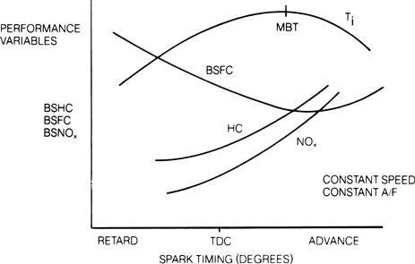
Figure 5.13 Typical variation of performance with spark timing.
Operation at or near MBT is desirable since this spark timing tends to optimize performance. This optimal spark timing varies with RPM. As will be explained, engine control strategy involves regulating fuel delivery at a stoichiometric mixture and varying ignition timing for optimized performance. However, there is yet another variable to be controlled, which assists the engine control system in meeting exhaust gas emission regulations.
Effect of Exhaust Gas Recirculation on Performance
Up to this point in the discussion, only the traditional calibration parameters of the engine (air/fuel ratio and spark timing) have been considered. However, by adding another control variable, the undesirable exhaust gas emission of NOx can be significantly reduced while maintaining a relatively high level of torque. This new control variable, exhaust gas recirculation (EGR), consists of recirculating a precisely controlled amount of exhaust gas into the intake. The engine control configuration depicted in Figure 5.5 shows that exhaust gas recirculation is a major subsystem of the overall control system. Its influence on emissions is shown in Figures 5.14 and 5.15 as a function of the percentage of exhaust gas in the intake. Figure 5.14 shows the dramatic reduction in NOx emission when plotted against air/fuel ratio, and Figure 5.15 shows the effect on performance variables as the percentage of EGR is increased. Note that the emission rate of NOx is most strongly influenced by EGR and decreases as the percentage of EGR increases. The HC emission rate increases with increasing EGR; however, for relatively low EGR percentages, the HC rate changes only slightly. Thus, a compromise EGR rate between NOx reduction and HC increase is possible in which the benefits of EGR on NOx reduction far offset the adverse effect on HC emissions. This compromise amount of EGR varies with engine configuration.
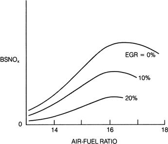
Figure 5.14 NOx emission as a function of air/fuel ratios at various EGR%.
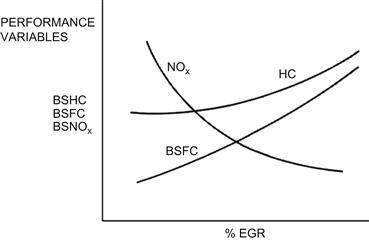
Figure 5.15 Influence of EGR on brake-specific performance variables.
The mechanism by which EGR affects NOx production is related to the peak combustion temperature. Roughly speaking, the NOx generation rate increases with increasing peak combustion temperature if all other variables remain fixed. Increasing EGR tends to lower this temperature; therefore, it tends to lower NOx generation. It should be noted that EGR, though relatively small, does influence the air partial pressure in the intake mixture. Compensation for this effect is required as explained later.
Exhaust Catalytic Converters
It is the task of the electronic control system to set the calibration for each engine-operating condition. There are many possible control strategies for setting the variables for any given engine, and each tends to have its own advantages and disadvantages. Moreover, each automobile manufacturer has a specific configuration that differs in certain details from competitive systems. However, this discussion is about a typical electronic control system that is highly representative of the systems for engines used by U.S. manufacturers. This typical system is one that has a catalytic converter in the exhaust system. Exhaust gases passed through this device are chemically altered in a way that reduces tailpipe emissions relative to engine output exhaust. Essentially, the catalytic converter reduces the concentration of undesirable exhaust gases coming out of the tailpipe relative to engine-out gases (the gases coming out of the exhaust manifold).
The EPA regulates only the exhaust gases that leave the tailpipe; therefore, if the catalytic converter reduces exhaust gas emission concentrations, the engine exhaust gas emissions at the exhaust manifold can be higher than the EPA requirements. This has the significant benefit of allowing engine calibration to be set for better performance than would be permitted if exhaust emissions in the engine exhaust manifold had to satisfy EPA regulations. This is the type of system that is chosen for the typical electronic engine control system.
Several types of catalytic converters are available for use on an automobile. The desired functions of a catalytic converter include
Oxidizing Catalytic Converter
The oxidizing catalytic converter (Figure 5.16) has been one of the more significant devices for controlling exhaust emissions since the era of emission control began. The purpose of the oxidizing catalyst (OC) is to increase the rate of chemical reaction, which initially takes place in the cylinder as the compressed air–fuel mixture burns, toward an exhaust gas that has complete oxidation of HC and CO to H2O and CO2.
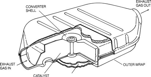
Figure 5.16 Catalytic converter configuration.
The extra oxygen required for this oxidation is often supplied by adding air to the exhaust stream from an engine-driven air pump. This air, called secondary air, is normally introduced into the exhaust manifold.
The most significant measure of the performance of the OC is its conversion efficiency,
![]() (22)
(22)
where Mo is the mass flow rate of gas that has been oxidized leaving the converter and Mic is the mass airflow rate of gas into the converter
The conversion efficiency of the OC depends on its temperature. Figure 5.17 shows the conversion efficiency (expressed as a percent) of a typical OC for both HC and CO as functions of temperature. Above about 300 degrees C, the efficiency approaches 98–99% for CO and more than 95% for HC.
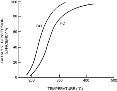
Figure 5.17 Oxidizing catalyst conversion efficiency versus temperature.
The Three-Way Catalyst
Another catalytic converter configuration that is extremely important for modern emission control systems is called the three-way catalyst (TWC). It uses a specific catalyst formulation containing platinum, palladium, and rhodium to reduce NOx and oxidize HC and CO all at the same time. It is called three way because it simultaneously reduces the concentration of all three major undesirable exhaust gases. The three-way catalyst uses a specific chemical design to reduce all three major emissions (HC, CO, and NOx) by approximately 90%.
The conversion efficiency of the TWC for the three exhaust gases depends mostly on the air/fuel ratio. Unfortunately, the air/fuel ratio for which NOx conversion efficiency is high, corresponds to a very low conversion efficiency for HC and CO and vice versa. However, as shown in Figure 5.18, there is a very narrow range of air/fuel ratio (called the window and shown as the lined region in Figure 5.18) in which an acceptable compromise exists between NOx and HC/CO conversion efficiencies. The conversion efficiencies within this window are sufficiently high to meet the very stringent EPA requirements established so far.

Figure 5.18 Conversion efficiency of a TWC vs. air/fuel.
Note that this window is only about 0.1 air/fuel ratio wide (± 0.05 air fuel ratio) and is centered at stoichiometry. (Recall that stoichiometry is the air/fuel ratio that would result in complete oxidation of all carbon and hydrogen in the fuel if burning in the cylinder were perfect; for gasoline, stoichiometry corresponds to an air/fuel ratio of 14.7.) This ratio and the concept of stoichiometry is extremely important in an electronic fuel controller. In fact, the primary function of most modern electronic fuel-control systems is to maintain average air/fuel ratio at stoichiometry. The operation of the three-way catalytic converter is adversely affected by lead. Thus, in automobiles using any catalyst, it is necessary to use lead-free fuel.
Controlling the average air/fuel ratio to the tolerances of the TWC window (for the full life requirement) requires accurate measurement of mass airflow rate and precise fuel delivery and is the primary function of the electronic engine control system. A modern electronic fuel-control system can meet these precise fuel requirements. In addition, it can maintain the necessary tolerances for government regulations for over 100,000 miles.
The fundamentals of any electronic engine control system are that it regulates the fuel/air mixture and ignition timing in response to an arbitrary driver input (via the throttle plate). The driver input includes the accelerator pedal position which ultimately determines the throttle position. The electronic engine control system directly determines a corresponding fuel quantity delivered to the engine which optimizes performance subject to a somewhat complex set of constraints. The constrained optimization involves compromises between the conflicting constraints of emission regulations and required fuel economy. As explained above, there are other control variables (e.g., spark timing EGR) that are part of the constrained optimization process.
Electronic Fuel-Control System
For an understanding of the configuration of an electronic fuel-control system, refer to the block diagram of Figure 5.19. The primary function of this fuel-control system is to determine the mass airflow rate accurately into the engine. Then the control system precisely regulates fuel delivery such that the ratio of the mass of air to the mass of fuel in each cylinder is as close as possible to stoichiometry (i.e., 14.7). The components of this block diagram are as follows:
1. throttle position sensor (TPS)
5. exhaust gas oxygen sensor (EGO)
6. engine coolant sensor (ECS)
7. engine position sensor (EPS)
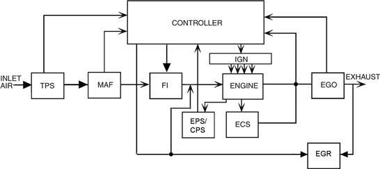
Figure 5.19 Electronic fuel-control configuration.
The EPS has the capability of measuring crankshaft angular speed (RPM) as well as crankshaft angular position when it is used in conjunction with a stable and precise electronic clock (in the controller) as explained in Chapter 6. The camshaft position sensor typically generates a timing pulse for each camshaft revolution (i.e., one complete engine cycle); the combination of EPS and CPS yields an unambiguous measurement of engine angular position (within each engine cycle) for each cylinder. The CPS sensor is required in a four-stroke/cycle engine since each cycle involves two complete crankshaft revolutions as explained above.
The signals from the various sensors enable the controller to determine the correct fuel flow in relation to the airflow to obtain the stoichiometric mixture. From this calculation, the correct fuel delivery is regulated via fuel injectors (FI). In addition, optimum ignition timing is determined and appropriate timing pulses are sent to the ignition control module (IGN).
The intake air passes through the individual pipes of the intake manifold to the various cylinders. The set of fuel injectors (one for each cylinder) are each normally located near the intake valve within the corresponding cylinder. As explained in Chapter 6, each fuel injector is an electrically operated valve that is (ideally) either fully open or fully closed. When the valve is closed, there is, of course, no fuel delivery. When the valve is open, fuel is delivered at a fixed rate as set by the fuel injector characteristics as well as fuel supply pressure. The amount of fuel delivered to each cylinder during engine cycle k (Mf(k)) is determined by the length of time τk that the fuel injector valve is open. This time is, in turn, computed in the engine controller to achieve the desired air/fuel ratio. Typically, the fuel injector open timing is set to coincide with the time that air is flowing into the cylinder during the intake stroke. However, at relatively low fuel delivery rates (e.g., near closed throttle), the control system must account for the relatively short opening and closing fuel injector dynamic transients response. The control system generates a pulsed electrical signal of sufficient amplitude to open the fuel injector valve. The duration of this pulse τk regulates the quantity of fuel such that the mass of fuel delivered (Mf) is given by
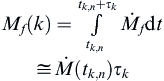 (23)
(23)
where ![]() is the fuel mass flow rate and tk,n the time of fuel delivery to cylinder n during engine cycle k.
is the fuel mass flow rate and tk,n the time of fuel delivery to cylinder n during engine cycle k.
It is assumed for this discussion that Mf(k) is the same for all cylinders during any engine cycle.
There is an important property of the catalytic converter that allows for momentary (very short term) fluctuations of the air/fuel ratio outside the narrow window. As the exhaust gases flow through the catalytic converter, they are actually in it for a short (but nonzero) amount of time, during which the conversions described above take place. Because of this time interval, the conversion efficiency is unaffected by rapid fluctuations above and below stoichiometry (and outside the window) as long as the average air/fuel ratio over time remains within the window centered at stoichiometry provided the fluctuations are rapid enough. A practical fuel-control system maintains the average mixture at stoichiometry but has minor (relatively rapid) fluctuations about the average, as explained below.
The electronic fuel-control system operates in two modes: open-loop and closed-loop. Recall the concepts for open-loop and closed-loop control as explained in Chapter 1. In the open-loop mode (also called feedforward), the mass airflow rate ![]() into the engine is measured. Then the fuel-control system determines the quantity of fuel (Mf) to be delivered to meet the required air/fuel ratio.
into the engine is measured. Then the fuel-control system determines the quantity of fuel (Mf) to be delivered to meet the required air/fuel ratio.
In the closed-loop control mode (also called feedback), a measurement of the controlled variable is provided to the controller (i.e., it is fed back) such that an error signal between the actual and desired values of the controlled variable is obtained. Then the controller generates an actuating signal that tends to reduce the error to zero.
In the case of fuel control, the desired variables to be measured are HC, CO, and NOx concentrations. Unfortunately, there is no cost-effective, practical sensor for such measurements that can be built into the car’s exhaust system. On the other hand, there is a relatively inexpensive sensor that gives an indirect measurement of HC, CO, and NOx concentrations. This sensor generates an output that depends on the concentration of residual oxygen in the exhaust after combustion. As will be explained in detail in Chapter 6, this sensor is called an exhaust gas oxygen (EGO) sensor. There it is shown that the EGO has evolved since its introduction in the earliest electronic control systems. For the purposes of the present chapter we consider the simplest model for an EGO sensor. In this simplified model, the EGO sensor output switches abruptly between two voltage levels depending on whether the input air/fuel ratio is richer than or leaner than stoichiometry. Such a sensor is appropriate for use in a limit-cycle type of closed-loop control. Although the EGO sensor is a switching-type sensor, it provides sufficient information to the controller to maintain the average air/fuel ratio over time at stoichiometry, thereby meeting the mixture requirements for optimum performance of the three-way catalytic converter.
In a typical modern electronic fuel-control system, the fuel delivery is partly open-loop and partly closed-loop. The open-loop portion of the fuel flow is determined by measurement of mass airflow. This portion of the control sets the air/fuel ratio at approximately stoichiometry. A closed-loop portion is added to the fuel delivery to ensure that time-average air/fuel ratio is at stoichiometry (within the tolerances of the window).
There are exceptions to the stoichiometric mixture setting during certain engine-operating conditions, including engine start, heavy acceleration, and deceleration. There are also exceptions due to ambient environmental conditions, particularly engine temperature as well as ambient air temperature and pressure. These conditions represent a very small fraction of the overall engine-operating times. They are discussed in Chapter 7, which explains the operation of a modern, practical digital electronic engine control system.
Engine Control Sequence
The step-by-step process of events in fuel control begins with engine start. During engine cranking the mixture is set rich by an amount depending on the engine temperature (measured via the engine coolant sensor), as explained in detail in Chapter 7. Generally speaking, the mixture is relatively rich for starting and operating a cold engine as compared with a warm engine. However, the discussion of this requirement is deferred to Chapter 7. Once the engine starts and until a specific set of conditions is satisfied, the engine control operates in the open-loop mode.
After combustion, the exhaust gases flow past the EGO sensor, through the TWC, and out the tailpipe. Once the EGO sensor has reached its operating temperature (typically a few seconds to about two minutes depending upon ambient conditions and the type of sensor used [see Chapter 6]), the EGO sensor signal is input to the controller and the system begins closed-loop operation.
Open-Loop Control
Fuel control for an electronically controlled engine operates open-loop any time the conditions are not met for closed-loop operation. Among many conditions (which are discussed in detail in Chapter 7) for closed-loop operations, there are some temperature requirements. After operating for a sufficiently long period after starting, a liquid-cooled automotive engine operates at a steady temperature.
However, an engine that is started cold initially operates in open-loop mode. This operating mode requires, at minimum, measurement of the mass airflow into the engine, and a measurement of RPM as well as measurement of coolant temperature. The mass airflow rate measurement in combination with RPM permits computation (by the engine controller) of the mass of air (Ma) drawn into each cylinder during intake for each engine cycle. The correct fuel mass (Mf) that is injected with the intake air is computed by the electronic controller:
![]() (24)
(24)
where rfa is the desired ratio of fuel to air.
For a fully warmed-up engine, this ratio is 1/14.7, which is about .068. That is, 1 lb of fuel is injected for each 14.7 lb of air, making the air/fuel ratio 14.7 (i.e., stoichiometry). The desired fuel/air ratio varies with temperature in a known way such that the correct value can be found from the measurement of coolant temperature. For a very cold engine, the mixture ratio can go as low as about 2 (i.e., ![]() ).
).
Theoretically, if there were no changes to the engine, the sensors, or the fuel injector, an engine control system could operate open-loop at all times. In practice, owing to errors in the calculation of Ma, variations in manufactured components, as well as to factors such as wear, the open-loop control would not be able to maintain the mixture at the desired air/fuel ratio if it were used alone. In order to maintain the very precise air/fuel mixture ratio required for emission control over the full life of the vehicle, the engine controller is operated in closed-loop mode for as much of the time as possible. Compensation for the open-loop mode variations above is possible via adaptive closed-loop control as explained in Chapter 7.
Closed-Loop Control
Referring to Figure 5.20, the control system in closed-loop mode operates as follows. For any given set of operating conditions, the fuel metering actuator provides fuel flow to produce an air/fuel ratio set by the controller output. This mixture is burned in the cylinder and the combustion products leave the engine through the exhaust pipe. The EGO sensor generates a feedback signal for the controller input that depends on the exhaust gas oxygen concentration. This concentration is a function of the intake air/fuel during the intake portion of the same cycle which is 1.5 crankshaft revolutions earlier than the time at which the EGO sensor output is measured.
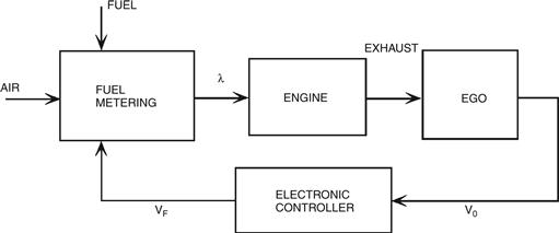
Figure 5.20 Simplified typical closed-loop fuel-control system block diagram.
One closed-loop control scheme that has been used in practice (i.e., limit-cycle control) results in the air/fuel ratio cycling around the desired set point of stoichiometry. The important parameters for this type of control include the amplitude and frequency of excursion away from the desired stoichiometric set point. Fortunately, the three-way catalytic converter’s characteristics are such that only the short-term time-average air/fuel ratio determines its performance. The variation in air/fuel ratio during the limit-cycle operation is so rapid that it has no effect on engine performance or emissions, provided that the average air/fuel ratio remains at stoichiometry.
Exhaust gas oxygen concentration
The EGO sensor, which provides feedback, will be explained in Chapter 6. In essence, the EGO generates an output signal that depends on the amount of oxygen in the exhaust. This oxygen level, in turn, depends on the air/fuel ratio entering the engine. The amount of oxygen is relatively low for rich mixtures and relatively high for lean mixtures. In terms of equivalence ratio (λ), recall that λ = 1 corresponds to stoichiometry, λ > 1 corresponds to a lean mixture with an air/fuel ratio greater than stoichiometry, and λ < 1 corresponds to a rich mixture with an air/fuel ratio less than stoichiometry. (The EGO sensor is sometimes called a lambda sensor.) Fuel entering each cylinder having a relatively lean mixture (i.e., excess oxygen) results in a relatively high oxygen concentration in the exhaust after combustion. Correspondingly, intake fuel and air having a relatively rich mixture (i.e., low oxygen) result in relatively low oxygen concentration in the exhaust.
For the purposes of the present chapter, a relatively simple continuous time model for an ideal EGO sensor output voltage Vo is given in Eqn (25):
![]() (25)
(25)
where td is the time delay from input mixture for a given engine cycle to the corresponding exhaust gases reaching the EGO sensor. This time delay which is about three-quarters of the period of an engine cycle varies inversely with engine RPM. The parameters V1 and V2 are derived from the pair of actual EGO sensor voltages for λ < 1 and λ > 1 (see Chapter 6) and are approximately
![]()
Although there are many potential control strategies for a switching-type sensor such as the EGO sensor, we will illustrate with a relatively straightforward example. Any control system incorporating a switching sensor (as characterized by the above model) will operate in a form of limit-cycle type of operation. As explained above, the fuel delivered to any given cylinder by its fuel injector during the kth engine cycle (Mf(k)) is proportional to the time interval (τF(k)) of its binary-valued control electrical signal VF(k) (see Figure 5.20). In our present example controller, the fuel injector (i.e., actuator) control voltage is given by
![]() (26)
(26)
where tk,n is the injection time during kth engine cycle for the nth cylinder.
The fuel injector duration τF(k) consists of an open-loop component τo(k) plus a closed-loop component τFc:
![]() (27)
(27)
where τo(k) is calculated based on ![]() measurement.
measurement.
Closed-Loop Operation
In the present example, the closed-loop portion of the pulse duration τF(k) for each cycle τFc(k) is a function of the equivalence ratio at the EGO sensor:
![]() (28)
(28)
whenever the mixture is lean of stoichiometry (i.e., λ > 1), the pulse duration increases by δτ from the previous cycle, thereby richening the mixture (and causing λ to decrease toward 1). Correspondingly, whenever λ < 1 (rich of stoichiometry), the pulse duration is decreased from cycle k to cycle k + 1. The open-loop portion of τF is a pulse whose duration τo(k) (called base pulse duration) is calculated to yield MF corresponding to stoichiometric mixture based upon mass airflow rate ![]() measurements. We illustrate the operation of this example fuel-control system in Figure 5.20.
measurements. We illustrate the operation of this example fuel-control system in Figure 5.20.
Lambda is used in the block diagram of Figure 5.20 to represent the equivalence ratio at the intake manifold. The exhaust gas oxygen concentration determines the EGO output voltage (Vo). The EGO output voltage abruptly switches between the lean and the rich levels as the air/fuel ratio crosses stoichiometry. The EGO sensor output voltage Vo is at its higher of two levels for a rich mixture and at its lower level for a lean mixture.
Reduced to its essential features, the engine control system operates as a limit-cycle controller in which the air/fuel ratio cycles up and down about the set point of stoichiometry, as shown by the idealized waveforms in Figure 5.21. The air/fuel ratio is either increasing or decreasing; it is never constant. The increase or decrease is determined by the EGO sensor output voltage. Whenever the EGO output voltage level indicates a lean mixture, the controller causes the air/fuel ratio to decrease, that is, to change in the direction of a rich mixture. On the other hand, whenever the EGO sensor output voltage indicates a rich mixture, the controller changes the air/fuel ratio in the direction of a lean mixture.

Figure 5.21 Simplified waveforms in a closed-loop fuel-control system.
The electronic fuel controller changes the mixture by changing the duration of the actuating signal to each fuel injector. Increasing this duration causes more fuel to be delivered, thereby causing the mixture to become richer. Correspondingly, decreasing this duration causes the mixture to become leaner. Figure 5.21b shows the fuel injector signal duration.
In Figure 5.21a the EGO sensor output voltage is at the higher of two levels over several time intervals, including 0–1 and 1.7–2.2. This high voltage indicates that the mixture is rich. The controller causes the pulse duration (Figure 5.21b) to decrease during this interval. At time 1 second, the EGO sensor voltage switches low, indicating a lean mixture. At this point the controller begins increasing the actuating time interval to tend toward a rich mixture. This increasing actuator interval continues until the EGO sensor switches high, causing the controller to decrease the fuel injector actuating interval. The process continues this way, cycling back and forth between rich and lean around stoichiometry.
The engine controller continuously computes the desired fuel injector actuation duration and maintains the current value in memory. At the appropriate time in the intake cycle, the controller reads the value of the fuel injector duration and generates a pulse of the correct duration to activate the proper fuel injector for the computed time interval τF.
One point that needs to be stressed at this juncture is that the air/fuel ratio deviates from stoichiometry. However, the catalytic converter will function as desired as long as the time-average air/fuel ratio is at stoichiometry. The controller continuously computes the average of the EGO sensor voltage. Ideally, the air/fuel ratio should spend as much time rich of stoichiometry as it does lean of stoichiometry. In the simplest case, the average EGO sensor voltage ![]() should be halfway between the rich and the lean values:
should be halfway between the rich and the lean values:
![]() (29)
(29)
Whenever this condition is not met, the controller adapts its computation of pulse duration (from EGO sensor voltage) to achieve the desired average stoichiometric mixture. Chapter 7 explains this adaptive control in more detail than is given here.
Frequency and deviation of the fuel controller
Recall from Chapter 1 that a limit-cycle controller regulates a system between two limits and that it has an oscillatory behavior; that is, the control variable oscillates about the set point or the desired value for the variable. The simplified fuel-controller operates in a limit-cycle mode and, as shown in Figure 5.21, the air/fuel ratio oscillates about stoichiometry (i.e., average air/fuel ratio is 14.7). The two end limits are determined by the rich and lean voltage levels of the EGO sensor, by the controller, and by the characteristics of the fuel metering actuator. The time necessary for the EGO sensor to sense a change in fuel metering is known as the transport delay. As engine speed increases, the transport delay decreases.
The frequency of oscillation fL of this limit-cycle control system is defined as the reciprocal of its period. The period of one complete cycle is denoted Tp, which is proportional to transport delay. Thus, the frequency of oscillation varies inversely with Tp and is given by
![]()
Furthermore, the transport delay varies inversely with engine speed (RPM). Therefore, the limit-cycle frequency is proportional to engine speed. This is depicted in Figure 5.22 for a representative typical engine.

Figure 5.22 Typical limit-cycle frequency versus RPM.
Another important aspect of limit-cycle operation is the maximum deviation of air/fuel ratio from stoichiometry. It is important to keep this deviation small because the net TWC conversion efficiency is optimum for stoichiometry. The maximum deviation typically corresponds to an air/fuel ratio deviation of about ![]() . Although the air/fuel ratio is constantly swinging up and down, the average value of deviation is held within
. Although the air/fuel ratio is constantly swinging up and down, the average value of deviation is held within ![]() of the 14.7:1 ratio. In addition, the limit-cycle frequency and deviation in a practical engine control are influenced by hysteresis in the transfer characteristics VF(λ) for an actual EGO sensor as discussed in Chapter 7.
of the 14.7:1 ratio. In addition, the limit-cycle frequency and deviation in a practical engine control are influenced by hysteresis in the transfer characteristics VF(λ) for an actual EGO sensor as discussed in Chapter 7.
Generally, the maximum deviation decreases with increasing engine speed because of the corresponding decrease in transport delay. The parameters of the control system are adjusted such that at the worst case the deviation is within the required acceptable limits for the TWC used.
The preceding discussion applies only to a simplified idealized fuel-control system. Chapter 7 explains the operation of practical electronic fuel-control systems in which the calculation of fuel injector duration is done numerically in a microprocessor-based engine control system.
Analysis of Intake Manifold Pressure
As explained earlier, fuel control is based on a measurement of mass airflow rate and on regulation of fuel flow to maintain a desired air/fuel ratio. Mass airflow measurement can be accomplished either directly or indirectly via computation based on measurement of other intake variables. For an understanding of this important measurement, it is helpful to consider the characteristics of the intake system, and the relationship between the relevant variables.
Figure 5.23 is a very simplified sketch of an intake manifold. In this simplified sketch, the engine is viewed as an air pump pumping air into the intake manifold. Whenever the engine is not running, no air is being pumped and the intake (MAP) is at atmospheric pressure. This is the highest intake MAP for a non-supercharged engine. (A supercharged engine has an external air pump called a supercharger.) When the engine is running, the airflow is impeded by the partially closed throttle plate. This reduces the pressure in the intake manifold so it is lower than atmospheric pressure; therefore, a partial vacuum exists in the intake.
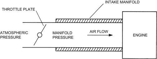
Figure 5.23 Simplified intake system configuration.
If the engine were a perfect air pump and if the throttle plate were tightly closed, a perfect vacuum could be created in the intake manifold. A perfect vacuum corresponds to zero absolute pressure. However, the engine is not a perfect pump and some air always leaks past the throttle plate. (In fact, some air must get past a closed throttle or the engine cannot idle.) Therefore, the intake MAP fluctuates during the stroke of each cylinder and as pumping is switched from one cylinder to the next.
Each cylinder contributes to the pumping action every second crankshaft revolution. For an N-cylinder engine, the frequency fp, in cycles per second, of the manifold pressure fluctuation for an engine running at a certain RPM is given by
![]()
Figure 5.24 shows manifold pressure fluctuations qualitatively as well as average MAP.

Figure 5.24 Intake manifold pressure fluctuations.
For a control system application, only average manifold pressure is required. The torque produced by an engine at a constant RPM is approximately proportional to the average value of MAP. The rapid fluctuations in instantaneous MAP are not of interest to the engine controller. Therefore, the manifold pressure measurement method should filter out the pressure fluctuations at frequency fp and measure only the average pressure. One way to achieve this filtering is to connect the MAP sensor to the intake manifold through a very small diameter tube. The rapid fluctuations in pressure do not pass through this tube, but the average pressure does. The MAP sensor output voltage then corresponds only to the average manifold pressure. Of course, electronic filtering of the MAP sensor voltage is also possible as explained in Chapter 1
Measuring Air Mass
A critically important aspect of fuel control is the requirement to measure the mass of air that is drawn into the cylinder (i.e., the air charge). The amount of fuel delivered can then be calculated such as to maintain the desired air/fuel ratio. There is no practically feasible way of measuring the mass of air in the cylinder directly. However, the air charge can be determined from the mass flow rate of air into the engine intake since all of this air eventually is distributed to the cylinders (ideally uniformly).
There are two methods of determining the mass flow rate of air into the engine. One method uses a single sensor that directly measures mass airflow rate. The operation of this sensor is explained in Chapter 6. The other method uses a number of sensors that provide data from which mass flow rate can be computed. This method is known as the speed-density method.
Speed-density method
The concept for this method is based on the mass density of air as illustrated in Figure 5.25a.
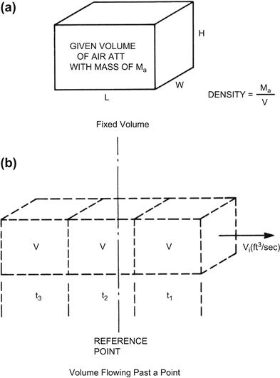
Figure 5.25 Volume flow rate calculation.
For a given volume of air (V) at a specific pressure (p) and temperature (T) having mass Ma, the density of the air (ρa) is given by
![]() (30)
(30)
This concept can be extended to moving air, as depicted in Figure 5.25b. Here air is assumed to be moving through a uniform tube (e.g., the intake pipe for an engine) past a reference point for a specific period of time. This is known as the volume flow rate.
Although the speed-density method of measuring ![]() has disappeared from contemporary engines, it is, perhaps, worthwhile to review it briefly in part because of its existence in older vehicles and in part to develop an understanding of this engine intake process. Earlier, it was shown that the mass airflow rate
has disappeared from contemporary engines, it is, perhaps, worthwhile to review it briefly in part because of its existence in older vehicles and in part to develop an understanding of this engine intake process. Earlier, it was shown that the mass airflow rate ![]() in the engine is given by
in the engine is given by
![]() (31)
(31)
where ρa is the density of the mixture of fuel air and water vapor:
![]() (32)
(32)
with pa being manifold absolute pressure, Ti being inlet air absolute temperature, and R being constant for and Vi is the volume flow rate.
In the above model, we neglect the relatively small contribution to manifold pressure of water vapor and assume that fuel is injected at the intake valve location, which is downstream from the throttle plate.
In Chapter 6, sensors are described for measuring pa (i.e., MAP sensor) and Ti (i.e., inlet air temperature sensor). Thus, the air density can readily be calculated based on measurements of these sensors. It was also shown earlier in this chapter in the discussion of volumetric efficiency that the air volume flow rate ![]() into the intake is given by
into the intake is given by
![]() (33)
(33)
where
![]()
The engine angular speed (N) is readily measured and the volumetric efficiency is normally measured during the engine mapping process. Tables of ev vs. throttle angle and RPM can be stored in memory for retrieval during a calculation of ![]() in the engine controller. Thus, via measurement and table look-up, the engine control has sufficient data to calculate (or at least to closely estimate)
in the engine controller. Thus, via measurement and table look-up, the engine control has sufficient data to calculate (or at least to closely estimate) ![]() from which fuel delivery quantities are readily computed.
from which fuel delivery quantities are readily computed.
Influence of Valve System on Volumetric Efficiency
For any given engine configuration, volumetric efficiency is determined by the intake manifold, the valve sizes, and locations, as well as the timing and profile of the cam lobe characteristics. The design of the cam lobe profile determines when the valves open and close and determines the maximum valve opening (lift). Any given cam profile is optimum only for a relatively narrow range of RPMs and throttle settings. Compromises are made between low-, high-, and mid-range RPMs as well as part throttle versus open or closed throttle.
Ideally, it would be desirable to vary valve timing and lift continuously as the engine operates so as to optimize volumetric efficiency. One technology exists for such variable valve timing (VVT) and is found in certain production vehicles. Variable valve timing is also called variable valve phasing (VVP) which is the preferred terminology in this book.
This technology involves separate camshafts for intake and exhaust valves. These two camshafts are driven via a mechanism that varies the relative timing for intake and exhaust. This mechanism (which includes an electromechanical actuator) and its operation are explained in Chapter 6. There it is shown that either (or both) intake and exhaust valve timing is varied relative to the engine cycle. The control strategy for regulating VVP is explained in Chapter 7.
In essence, the exhaust valve is open primarily during the exhaust stroke and that the intake valve is open primarily during the intake stroke. Typically in automotive engines, the exhaust valve remains open during the initial portion of the intake valve-opening period. The crankshaft angle over which the two valves are both open (or partially open) is called overlap. Valve overlap permits exhaust action to assist the intake and improve volumetric efficiency. It also permits some exhaust gas to be mixed with intake gases such the EGR system is at least partially implemented by engine pumping processes. In a variable cam phasing system, this overlap is minimum at idle and varies with operating conditions to optimize emissions and performance. This topic is discussed in detail in Chapters 6 and 7.
Including EGR
Calculating ![]() is relatively straightforward in a computer-based control system. Another factor must be taken into account in determining mass airflow rate. Exhaust gas recirculation requires that a certain portion of the charge into the cylinders be exhaust gas. Because of this, a portion of the displacement VD is exhaust gas. Therefore, the volume flow rate of EGR must be known. A valve-positioning sensor in the EGR valve can be calibrated to provide the flow rate.
is relatively straightforward in a computer-based control system. Another factor must be taken into account in determining mass airflow rate. Exhaust gas recirculation requires that a certain portion of the charge into the cylinders be exhaust gas. Because of this, a portion of the displacement VD is exhaust gas. Therefore, the volume flow rate of EGR must be known. A valve-positioning sensor in the EGR valve can be calibrated to provide the flow rate.
From this information for the speed-density method of calculating ![]() , the true volume flow rate of air,
, the true volume flow rate of air, ![]() , can be determined by subtracting the volume flow rate of EGR
, can be determined by subtracting the volume flow rate of EGR ![]() from
from ![]() . The total cylinder air charge rate
. The total cylinder air charge rate ![]() is thus given as follows:
is thus given as follows:
![]() (34)
(34)
The volume flow rate of EGR is known from the position of the EGR valve and from engine-operating conditions, as explained in Chapter 7.
Substituting the equation for ![]() , the volume flow rate of air is
, the volume flow rate of air is
![]() (35)
(35)
Knowing ![]() and the density ρa gives the mass flow rate of air
and the density ρa gives the mass flow rate of air ![]() as follows:
as follows:
![]() (36)
(36)
Knowing ![]() the stoichiometric mass flow rate for the fuel,
the stoichiometric mass flow rate for the fuel, ![]() , can be calculated as follows:
, can be calculated as follows:
![]() (37)
(37)
Continuing with the discussion of the speed-density method for measuring ![]() , it is the function of the fuel metering actuator to set the fuel mass flow rate at this desired value based on the values of
, it is the function of the fuel metering actuator to set the fuel mass flow rate at this desired value based on the values of ![]() and pa. The control system continuously calculates
and pa. The control system continuously calculates ![]() from
from ![]() and ρa at the temperature and manifold pressure involved, and generates an output electrical signal to operate the fuel injectors to produce a stoichiometric mass fuel rate. For a practical engine control system, it completes such a measurement, computation, and control signal generation at least once for each cylinder firing.
and ρa at the temperature and manifold pressure involved, and generates an output electrical signal to operate the fuel injectors to produce a stoichiometric mass fuel rate. For a practical engine control system, it completes such a measurement, computation, and control signal generation at least once for each cylinder firing.
Idle Speed Control
The operation of an automotive engine at idle involves a special consideration. Under idle conditions, there is no input to the throttle from the driver via the accelerator pedal. The engine must produce exactly the torque required to balance all applied load torques from the transmission and any accessories as well as internal friction and pumping torques in order to run at a steady idle angular speed (RPM). Certain load torques occur as a result of driver action (e.g., change in the transmission selector from park or neutral to drive or reverse as well as switching electrical loads). However, certain other load torques occur without a direct driver command (e.g., air conditioner clutch actuation).
As in all engine-operating modes, the torque produced by the engine at idle is determined by the mass flow rate of intake air. The electronic fuel control regulates fuel flow to maintain stoichiometry as long as the engine is fully warmed and may briefly regulate fuel to somewhat richer than stoichiometry during cold starts. Normally the electronic engine control is intended to operate the engine at a fixed RPM regardless of load. It does this by regulating mass airflow with the throttle command from the driver at zero. The airflow required to maintain the desired idle RPM must enter the engine via the throttle assembly with the throttle at a small but nonzero angle. Alternatively, some engines are equipped with a special air passage that bypasses the throttle plate. For either method an actuator is required to enable the electronic engine control system to regulate the idle mass airflow rate. Chapter 6 discusses various actuators having application for idle airflow control. For the present discussion, we assume a model for the idle mass airflow rate that is representative of the practical actuator configurations discussed in Chapter 6. (Note: In the following analysis, the subscript I is included for all variables and parameters to emphasize that the present system refers to idle speed control.)
Regardless of the idle air bypass configuration, the mass airflow at idle condition (which we denote ![]() ) is proportional to the displacement of a movable element that regulates the size of the aperture through which the idle air flows (e.g., the throttle angle θT or its equivalent xT in an idle bypass structure). For the purposes of the present discussion, we assume that the engine indicated torque at idle TiI is given by
) is proportional to the displacement of a movable element that regulates the size of the aperture through which the idle air flows (e.g., the throttle angle θT or its equivalent xT in an idle bypass structure). For the purposes of the present discussion, we assume that the engine indicated torque at idle TiI is given by
![]() (38)
(38)
where KI is the constant for the idle air system; we further assume that ![]() varies linearly with the position of the idle bypass variable xI:
varies linearly with the position of the idle bypass variable xI:
![]() (39)
(39)
where xI is the opening in the idle bypass passage way and Km the constant for this structure.
Typically, the movable element in the idle air bypass structure incorporates a spring that acts to hold xI = 0 in the absence of any actuation. The actuation force (or torque) acts on the force (torque) of this spring as well as the internal force (torque) in accelerating the mass mI (or moment of inertia for rotating air bypass configuration) of the movable elements and the friction force (torque). We assume, for the present, a linear model for the actuator motion:
![]() (40)
(40)
where dI is the viscous friction constant, kI the spring rate of restoring spring, u the actuator input signal, and Ka the actuator constant.
It is also necessary for this discussion of idle speed control to have a model for the relationship between indicated torque and engine angular speed at idle. To avoid potential confusion with other frequency variables, we adapt the notation ΩI for the crankshaft angular speed of idle (rad/sec). This variable is given by
![]() (41)
(41)
where
![]()
In general for relatively small changes in ΩI, the load torques (including friction pumping torques) can be represented by the following linear model:
![]()
where Re is essentially constant for a given engine/load configuration at a particular operating temperature. The indicated torque at idle TiI has the following approximate linear model:
![]() (42)
(42)
where Je is the moment of inertia of engine and load rotating components.
Using the Laplace transform methods of Chapter 1, it is possible to obtain the engine transfer function at idle HeI(s):
![]() (43)
(43)
![]() (44)
(44)
Similarly, the transfer function for the idle speed actuator dynamics HaI(s) is given by
 (45)
(45)
![]()
![]()
These transfer functions can be combined to yield the transfer function (in standard form) of the idle speed control “plant” HpI(s):
![]() (46)
(46)
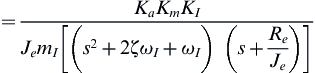 (47)
(47)
where u is the control variable that is sent to the actuator.
Open-loop control of idle speed is not practical owing to the large variations in load as well as parameter changes due to variations in operating environmental conditions. On the other hand, closed-loop control is well suited to regulating idle speed to a desired value. Figure 5.26 is a block diagram of such an idle speed control system.
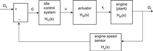
Figure 5.26 Idle speed control system block diagram.
Using the analysis procedures of Chapter 1 and denoting the idle speed set point Ωs, it can be shown that the idle speed control closed-loop transfer function HCLI is given by
 (48)
(48)
where HcI is the transfer function for the idle speed controller and Hs(s) the transfer function for the crankshaft speed sensor.
In Chapter 1, there were three control strategies introduced: P, PI, and PID. Of these, the proportional only (P) is undesirable since it has a nonzero steady-state error between ΩI and its desired value (Ωs). It was also shown in Chapter 1 that a proportional–integral (PI) control had zero steady-state error but could potentially yield an unstable closed-loop system. However, depending upon the system parameters there are ranges of values for both the proportional gain (Kp) and integral gain (KI) for which stable operation is possible and for which the idle speed control system has acceptable performance. The controller transfer function for PI control is given by
![]() (49)
(49)
For the purpose of illustrating exemplary idle speed control performance, we assume the following set of parameters:
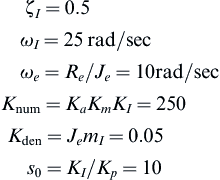
The forward transfer function HF(s) is defined by the following expression:
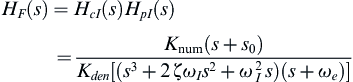 (50)
(50)
The present analysis is simplified by assuming a perfect angular speed sensor such that Hs(s) = 1. In this case, the closed-loop idle speed control transfer function (HCLI(s)) is given by
![]() (51)
(51)
The influence of proportional gain on stability of this closed-loop idle speed control can be evaluated via root locus techniques as explained in Chapter 1. Figure 5.27 is a plot of the root locus for this idle speed control with the assumed parameters.
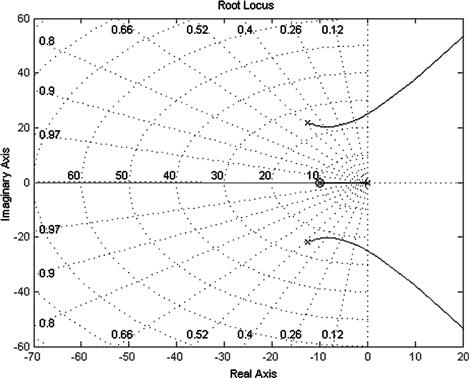
Figure 5.27 Root locus for idle speed control.
It can be seen from this figure that the closed-loop poles all begin in the left half complex plane and are all stable. However, as Kp increases, a pair of poles cross over into the right half complex plane and are unstable. Using the MATLAB “data cursor” function under the tools bar on the root locus plot, it can be seen that for Kp = 1.2, the poles that migrate to the right-hand side of the complex plane are stable and have a damping ratio of about 25%.
Using this value for Kp (i.e., Kp = 1.2), the closed-loop dynamic response for the system was examined by commanding a step change in RPM from an initial 550 RPM to 600 RPM at t = 0.5 s. Figure 5.28 is a plot of the dynamic response of engine idle speed (in RPM) to this command input.

Figure 5.28 Step response of idle speed control.
It can be seen that the idle speed reaches the command RPM after a brief transient response with zero steady-state error.
The parameters used in this idle speed control simulation are not necessarily representative of any particular engine. Rather they have been chosen to illustrate characteristics of this important engine control function. In Chapter 7 where digital engine (powertrain) control is discussed, a discrete time control is modeled.
Electronic Ignition
The engine ignition system exists solely to provide an electric spark to ignite the mixture in the cylinder. As explained earlier in this chapter, the engine performance is strongly influenced by the spark timing relative to the engine position during the compression stroke (see also Chapter 1). The spark advance (relative to TDC) is determined in the electronic engine control based on a number of measurements made by sensors. As will be explained in Chapter 7, the optimum spark advance varies with the intake manifold pressure, RPM, and temperature.
However, in order to generate a spark at the correct spark advance, the electronic engine control must have a measurement of the crankshaft angular position within an engine cycle. The engine position measurement is determined by a sensor coupled to the camshaft and another coupled to the crankshaft.
Electronic ignition can be implemented as part of an integrated system or as a stand-alone ignition system. A block diagram for the latter system is shown in Figure 5.29.
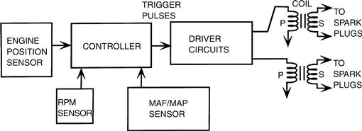
Figure 5.29 Electronic ignition system configuration.
Based on measurements from the sensors for engine position, mass airflow or manifold pressure, and RPM, the electronic controller computes the correct spark advance for each cylinder. At the appropriate time, the controller sends a trigger signal to the driver circuits, thereby initiating spark. Before the spark occurs, the driver circuit sends a relatively large current through the primary (P) of the coil. When the spark is to occur, a trigger pulse is sent to the driver circuit to interrupt the current in the primary. A very high voltage is induced at this time in the secondary (S) of the coil. The physical mechanism by which this interrupted primary current causes the high voltage in the coil secondary windings is explained in Chapter 6. This high voltage is applied to the spark plugs, causing them to fire. In those cases for which a coil is associated with two cylinders, one of the two cylinders will be in this compression stroke. Combustion will occur in this cylinder, resulting in power delivery during its power stroke. The other cylinder will be in its exhaust stroke and the spark will have no effect. Most engines have an even number of cylinders and there can be a separate driver circuit and coil for each pair of cylinders.
Before proceeding with a discussion of contemporary discrete-time digital control of the complete powertrain, however, it is necessary to explain and develop models for the critically important components of a control system: sensors and actuators. Chapter 6 is devoted to these important components.