Chapter 8
Vehicle-Motion Controls
Chapter Outline
Representative Cruise Control System
Hardware Implementation Issues
Stepper Motor-based Actuator Electronics
Variable Damping via Variable Strut Fluid Viscosity
The term vehicle motion refers to the translation along and rotation about all three axes (i.e. longitudinal, lateral, and vertical) for a vehicle. By the term longitudinal axis, we mean the axis that is parallel to the ground (vehicle at rest) on a horizontal plane along the length of the car. The lateral axis is orthogonal to the longitudinal axis and is also parallel to the ground (vehicle at rest). The vertical axis is orthogonal to both the longitudinal and lateral axes.
Rotations of the vehicle around these three axes correspond to angular displacement of the car body in roll, yaw, and pitch. Roll refers to angular displacement about the longitudinal axis; yaw refers to angular displacement about the vertical axis; and pitch refers to angular displacement about the lateral axis.
In characterizing the vehicle dynamic motion, it is common practice to define a body-centered Cartesian coordinate system in which the x-axis is the longitudinal axis with positive forward. The y-axis is the lateral axis and is taken as the lateral axis with the positive sense to the right-hand side. The vertical axis is taken as the z-axis with the positive sense up.
The vehicle dynamic motion is represented as displacement, velocity, and acceleration of the vehicle relative to an earth-centered, earth-fixed (ECEF) inertial coordinate system (as will be explained later in this chapter) in response to forces acting on it. Although strictly speaking, the ECEF coordinate system is not truly an inertial reference, with respect to the types of motion of interest in most vehicle dynamics it is essentially an inertial reference system.
Electronic controls have been recently developed with the capability of regulating the motion along and about all three axes. Individual car models employ various selected combinations of these controls. This chapter discusses motion control electronics beginning with control of motion along the longitudinal axis in the form of a cruise control system.
The forces and moments/torque that influence vehicle motion along the longitudinal axis include those due to the powertrain (including, in selected models, traction control), the brakes, the aerodynamic drag, and tire-rolling resistance, as well as the influence of gravity when the car is moving on a road with a nonzero inclination (or grade). In a traditional cruise control system, the tractive force due to the powertrain is balanced against all resisting forces to maintain a constant speed. In an advanced cruise control system, brakes are also automatically applied as required to maintain speed when going down a hill of sufficiently steep grade. Longitudinal vehicle motion refers to translation of the vehicle in an ECEF y,z-plane.
Representative Cruise Control System
Automotive cruise control is an excellent example of the type of electronic feedback control system that was discussed in general terms in Chapter 1. Recall that the components of a control system include the plant, or system being controlled, and a sensor for measuring the plant variable being regulated. It also includes an electronic control system that receives inputs in the form of the desired value of the regulated variable and the measured value of that variable from the sensor. The control system generates an error signal constituting the difference between the desired and actual values of this variable. It then generates an output from this error signal that drives an electromechanical actuator. The actuator controls the input to the plant in such a way that the regulated plant variable is moved toward the desired value.
We begin with a simplified cruise control for a vehicle traveling along a straight road (along the x axis in our ECEF coordinate system). In the case of a cruise control, the variable being regulated is the vehicle speed:
![]()
where x is the translation of the vehicle in the ECEF frame.
The driver manually sets the car speed at the desired value via the accelerator pedal. Upon reaching the desired speed (Vd), the driver activates a momentary contact switch that sets that speed as the command input to the control system. From that point on, the cruise control system maintains the desired speed automatically by operating the throttle via a throttle actuator.
Under normal driving circumstances, the total external forces acting on the vehicle are such that a net positive traction force (from the powertrain) is required to maintain a constant vehicle speed. The total external forces acting on the vehicle include rolling resistance of the tires, aerodynamic drag, and a component of vehicle weight whenever the vehicle is traveling on a road with a slope relative to level. However, when the car is on a downward sloping road of sufficient grade, drag and tire-rolling resistance are insufficient to prevent vehicle acceleration (i.e. ![]() ) and maintaining a constant vehicle speed requires a negative tractive force that the powertrain cannot deliver. In this case, the car will accelerate unless brakes are applied. For our initial discussion, we assume this latter condition does not occur and that no braking is required. It is further assumed that the powertrain has sufficient power capability of maintaining constant vehicle speed on an up-sloping grade.
) and maintaining a constant vehicle speed requires a negative tractive force that the powertrain cannot deliver. In this case, the car will accelerate unless brakes are applied. For our initial discussion, we assume this latter condition does not occur and that no braking is required. It is further assumed that the powertrain has sufficient power capability of maintaining constant vehicle speed on an up-sloping grade.
The plant being controlled consists of the powertrain (i.e. engine and drivetrain), which propels the vehicle through the drive axles and wheels. As described above, the load on this plant includes friction and aerodynamic drag as well as a portion of the vehicle weight when the car is going up- and down-hills.
For an understanding of the dynamic performance of a cruise control, it is helpful to develop a model for vehicle motion along a road. The basic performance of a cruise control can be presented with a few simplifying assumptions. In the interest of safety a typical cruise control cannot be activated below a certain speed (e.g. 40 mph). For the purposes of presenting the present somewhat simplified model, it is assumed that the vehicle is traveling along a straight road at a cruise speed with the automatic transmission in torque converter lock-up mode (see Chapter 7). This assumption removes some powertrain dynamics from the model. It is further assumed that the transmission is in direct drive such that its gear ratio is 1. The total gear ratio is given by the differential/transaxle gear ratio gA where typically ![]() . Under this assumption, the torque applied to the drive wheels Tw is given by
. Under this assumption, the torque applied to the drive wheels Tw is given by
![]() (1)
(1)
where Tb is the engine brake torque.
The cruise control system employs an actuator that moves the throttle in response to the control signal. Of course whenever the cruise control is disabled, this actuator must release control of the throttle such that the driver controls throttle angular position via the accelerator pedal and associated linkage. Except for roads with relatively steep grades, normally, once cruise control is activated relatively small, changes in throttle position are required to maintain selected vehicle speed. For our simplified model we assume that Tb varies linearly with cruise control output electrical signal u:
![]() (2)
(2)
where Ka is a constant for the engine/throttle actuator. This assumption, though not strictly valid, permits a system performance analysis using the discussion of linear control theory of Chapter 1 without any serious loss of generality.
A vehicle traveling along a straight road at speed V experiences forces due to the wheel torque Tw, aerodynamic drag D tire-rolling resistance Frr, and inertial forces. A dynamic model for the vehicle longitudinal (i.e. along the direction of travel and vehicle fore/aft axis) is given by
![]() (3)
(3)
where
rw = drive wheel effective radius
μr = coefficient of tire-rolling resistance
θ = angle of the road surface relative to a horizontal plane
Vw = the component of wind along vehicle longitudinal axis (positive for head wind negative for tail wind).
In specifying a drag coefficient for a car, it is necessary to specify a reference area. Although the choice of Sref is somewhat arbitrary, conventional practice takes the largest vehicle cross-sectional area projected in a body y,z-plane. In the above nonlinear differential Eqn (3), the first term on the right-hand side (RHS) is the force acting on the vehicle due to the applied road torque acting at the tire/road interface due to the powertrain. The second term on the RHS is the component of force along the vehicle axis due to its weight and any road slope expressed by θ.
For a car traveling at constant cruise speed VC (i.e. ![]() ) along a level, horizontal road (i.e. θ = 0) with zero wind, the differential equation above reduces to an algebraic expression in terms of the engine brake torque and speed V:
) along a level, horizontal road (i.e. θ = 0) with zero wind, the differential equation above reduces to an algebraic expression in terms of the engine brake torque and speed V:
![]() (4)
(4)
This equation permits a determination of engine brake torque vs. cruise speed for a level road.
If the vehicle is traveling at a steady speed along a hill with slope angle θ, then the Tb is determined from the following equation:
![]() (5)
(5)
For the operation of the cruise control system, it is normally sufficient to model vehicle dynamics with a linearized version of the nonlinear differential equation. The drag term can be linearized by representing vehicle instantaneous speed (V(t)) with the approximate model assuming for simplicity that Vw = 0:
![]() (6)
(6)
![]()
where DC is the drag at speed VC:
![]()
![]()
where KD is a constant for a given initial steady cruise speed VC and constant ρ.
In modeling the cruise control system, it is helpful to consider the influence of road grade (θ) as a disturbance. This disturbance can be linearized to a close approximation by the substitution (provided that the slope of the hill is sufficiently small):
![]()
The linearized equation of motion is given by
![]() (7)
(7)
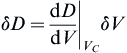
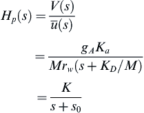
The operational transfer function Hp(s) for the “plant” for zero disturbance (i.e., θ = 0) is given by
 (8)
(8)
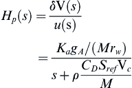
The configuration for a representative automotive cruise control is shown in Figure 8.1.
Figure 8.1 Cruise control configuration.
When the vehicle reaches the desired speed under normal driver accelerator pedal regulation of the throttle, to activate cruise control at that speed the driver pushes a momentary contact switch thereby setting the command speed in the controller. At this point, control of the throttle position is via the cruise control actuator. The momentary contact (pushbutton) switch that sets the command speed is denoted S1 in Figure 8.1.
Also shown in this figure is a disable switch that completely disengages the cruise control system from the power supply such that throttle control reverts back to the accelerator pedal. This switch is denoted S2 in Figure 8.1 and is a safety feature. In an actual cruise control system, the disable function can be activated in a variety of ways, including the master power switch for the cruise control system and a brake pedal-activated switch that disables the cruise control any time that the brake pedal is moved from its rest position. The throttle actuator opens and closes the throttle in response to the error between the desired and actual speed. Whenever the actual speed is less than the desired speed, the throttle opening is increased by the actuator, which increases vehicle speed, until the error is zero at which point the throttle opening remains fixed until either a disturbance occurs or the driver calls for a new desired speed.
A block diagram of a cruise control system is shown in Figure 8.2. In the cruise control depicted in this figure, a proportional integral (PI) control strategy has been assumed. Before the advent of digital cruise control, there were a variety of analog systems which had a proportional-only (P) control law. Nevertheless, the PI controller is representative of good design for such a control system since it can reduce steady-state speed errors to zero (as explained in Chapter 1). In this strategy, an error e is formed by subtracting (electronically) the actual speed V from the desired speed Vd:
![]() (9)
(9)
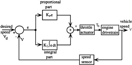
Figure 8.2 Cruise control block diagram.
It should be noted that the speed differential from Vc is the negative of the error (i.e. ![]() ). The controller then electronically generates the actuator signal by combining a term proportional to the error (Kpe) and a term proportional to the integral of the error:
). The controller then electronically generates the actuator signal by combining a term proportional to the error (Kpe) and a term proportional to the integral of the error:
![]() (10)
(10)
The actuator signal u is given by
![]() (11)
(11)
Operation of the system can be understood by considering the operation of a PI controller. We assume that the driver has reached the desired speed (say, 60 mph) and activated the speed set switch. The car is initially traveling on a level road at the desired speed. Then at some point it encounters a long hill with a steady positive slope (i.e. a hill going up).
The control signal at the output of the PI controller u is given by
![]() (12)
(12)
It is consistent with the linearized approximation to model the change in brake torque δTb due to actuator change in throttle position in response to the control signal u as linear in the control signal (as presented earlier):
![]()
where Ka is a constant for the throttle actuator–engine combination. With the above models and notation, the vehicle dynamic equation of motion becomes
 (13)
(13)
Taking the Laplace transform of the above equation and solving for the speed differential yield
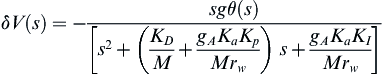 (14)
(14)
A computer simulation of this simplified cruise control was done for a step change in grade of θ = 0.03 starting at 2 s into the simulation for the following parameters in English units:
The simulation was done for the PI control but for reference purposes was also run for KI = 0 (i.e. a proportional-only control). Figure 8.3 shows the response for the car initially traveling under cruise control at 60 MPH. At time t = 2 s a hill of steady 5% (i.e. θ = 0.05) grade occurs (for the particular gains chosen). The dashed curve is the response of proportional-only control. Note that the speed drops down to a steady 53 MPH for the controller. The solid curve depicts the vehicle speed for the preferred PI control. Except for a brief overshoot, this control returns the vehicle speed to the set point of 60 MPH in a few seconds. It should be noted that the P-only control performance can be improved by increasing Kp (provided the system satisfies stability robustness criteria (see Chapter 1)).
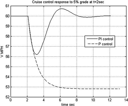
Figure 8.3 Cruise control speed performance.
The response characteristics of a PI controller depend strongly on the choice of the gain parameters Kp and KI. It is possible to select values for these parameters to increase the rate at which the system responds to disturbance. If this rate is increased too much, however, overshoot will increase and stability robustness (e.g. gain/phase margins) generally is reduced. As explained in Chapter 1, the amplitude of the speed error oscillations decreases by an amount determined by a parameter called the damping ratio. The damping ratio that produces the fastest response without overshoot is called critical damping.
The importance of these performance curves of Figure 8.3 is that they demonstrate how the performance of a cruise control system is affected by the controller gains. These gains are simply parameters that are contained in the control system. They determine the relationship between the error, the integral of the error, and the actuator control signal.
Usually a control system designer attempts to balance the proportional and integral control gains so that the system is optimally damped. However, because of system characteristics, in many cases, it is impossible, impractical, or inefficient to achieve the optimal time response and therefore another response is chosen. The control system should cause Tb to respond quickly and accurately to the command speed, but should not overtax the engine in the process. Therefore, the system designer chooses the control electronics that provide the following system qualities:
Digital Cruise Control
The explanation of the operation of cruise control thus far has been based on a continuous time formulation of the problem. This formulation correctly describes the concept for cruise control regardless of whether the implementation is by analog or digital electronics. Cruise control is now mostly implemented digitally using a microprocessor-based controller. For such a system, proportional and integral control computations are performed numerically in the computer. The digital cruise control is inherently a discrete time system with samples of the vehicle speed taken at integer multiples of the sample period Ts.
The block diagram for a representative digital cruise control is depicted in Figure 8.4.
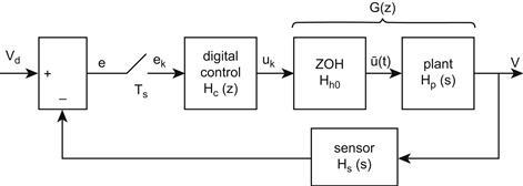
Figure 8.4 Digital speed control block diagram.
The plant variable being controlled is its forward speed V. The desired speed or set point for the controller is denoted Vd. The model for the plant as represented by its transfer function Hp(s) is taken to be the same as that developed above for the analog version of the cruise control. However, the actuator signal which is the ZOH output ![]() is a piecewise continuous signal (see Chapter 2):
is a piecewise continuous signal (see Chapter 2):
 (15)
(15)
![]()
![]()
Using the same parameters as were used for the analog version of the cruise control, this model is given numerically by the following transfer function:
![]() (16)
(16)
As explained in Chapter 2, the z-transfer function for the combination of ZOH and plant (G(z)) is given by
![]() (17)
(17)
From the methods of Chapter 2, the z-transform above can be found by expanding Hp(s)/s in a partial fraction series and then using the tables of Chapter 2. Then it is left as an exercise to show that for sample period Ts = 0.01 s, G(z) is given by
![]() (18)
(18)
where
The continuous time PI control law is given by
![]() (19)
(19)
In Chapter 7 under the section discussing control of variable valve phasing, it was shown that one discrete time z-transform of the integral term (using the trapezoidal integration rate) is given by
![]()
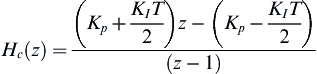
The z-operational transfer function for the controller is given by
![]() (20)
(20)
![]()
 (21)
(21)
Using the same gains (Kp = 10 and KI = 50) as for the continuous time control, one obtains
![]() (22)
(22)
Chapter 2 also showed that the forward path z-transfer function HF(z) for a discrete time control system as shown in Figure 8.4 is given by
 (23)
(23)
Assuming an ideal sensor for which Hs(s) = 1, the closed-loop gain z-transform function HCL(z) is given by
 (24)
(24)
The poles of this closed-loop transfer function are
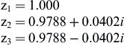
Since all poles are either on or inside the unit circle ![]() , the closed-loop cruise control system is stable.
, the closed-loop cruise control system is stable.
The dynamic response for this discrete time cruise control system can be found by evaluating its response to a step change in the input. Assume that the vehicle is cruising at a steady 60 MPH. Then, at t = 2 s (i.e., at sample k1 where k1 = 200), the cruise control set point is changed by a step increase of 10 to 70 MPH. This system set point is given by
![]() (25)
(25)
The z-transform for this system input is given by
![]() (26)
(26)
The output z-transform V(z) is given by
![]() (27)
(27)
The vehicle speed Vk at times tk is found by taking the inverse z-transform of V(z). Using the partial fraction expansion method of Chapter 2, the time response at t = tk is shown in Figure 8.5.

Figure 8.5 Response of digital cruise control to step change in set speed.
The speed is constant until k = k1 where t(k1) = 2 s and then increases with a relatively small overshoot approaching the final set point value of 70 MPH.
We consider next the implementation of the digital cruise control system in actual hardware. The vehicle speed sensor and the actuator are analog and can either be modeled as continuous or discrete time devices (examples of each are discussed below) and the control system is digital. When the car reaches the desired speed, Vd, the driver activates the speed set switch. At this time, the output of the vehicle speed sensor is sampled, converted to a digital value and transferred to a storage register. This is the set point for the controller.
Hardware Implementation Issues
The computer continuously reads the actual vehicle speed, V, and generates an error, en, at the sample time, tn:
![]()
A control signal, un, is computed that has the following form:
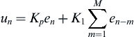 (28)
(28)
This sum, which is computed in the cruise control computer, is then multiplied by the integral gain KI and added to the most recent error multiplied by the proportional gain Kp to form the control signal. The computed discrete time control signal ![]() then must be converted to a piecewise continuous form
then must be converted to a piecewise continuous form ![]() suitable to operate the actuator (via a ZOH). It should be noted that
suitable to operate the actuator (via a ZOH). It should be noted that ![]() corresponds to the control signal u for the continuous time linear cruise control above. The correct form for this signal is discussed below in conjunction with the throttle actuator configuration.
corresponds to the control signal u for the continuous time linear cruise control above. The correct form for this signal is discussed below in conjunction with the throttle actuator configuration.
The operation of the cruise control system can be further understood by examining the vehicle speed sensor and the actuator in detail. Figure 8.6a is a sketch of a sensor configuration suitable for vehicle speed measurement.
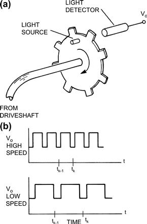
Figure 8.6 Example speed sensor configuration.
In a representative vehicle speed measurement system, the vehicle speed information is mechanically coupled to the speed sensor by a flexible cable coming from the driveshaft, which rotates at an angular speed proportional to vehicle speed. A speed sensor driven by this cable generates a pulsed electrical signal (Figure 8.6b) that is processed by the computer to obtain a digital measurement of speed.
A speed sensor can be implemented magnetically or optically. The magnetic speed sensor was discussed in Chapter 6, so we hypothesize an optical sensor for the purposes of this discussion. For the hypothetical optical sensor, a flexible cable drives a slotted disk that rotates between a light source and a light detector. The placement of the source, disk, and detector is such that the slotted disk interrupts or passes the light from source to detector, depending on whether a slot is in the line of sight from source to detector. The light detector produces an output voltage whenever a pulse of light from the light source passes through a slot to the detector. The number of pulses generated per second is proportional to the number of slots in the disk and the vehicle speed:
![]()
where f is the frequency in pulses per second, N is the number of slots in the sensor disk,
V is the vehicle speed, K is the proportionality constant that accounts for differential gear ratio and wheel size.
The sampled pulse frequency fk is computed from measurements of the time of each low to high transition denoted tk in Figure 8.6b:
![]()
The output pulses are passed through a sample gate to a binary counter (Figure 8.7).
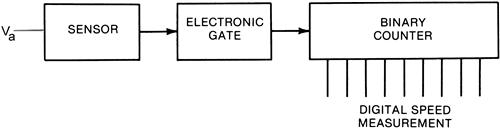
Figure 8.7 Digital speed measurement system.
The gate is an electronic switch that either passes the pulses to the counter or blocks their passage depending on whether the switch is closed or open. The time interval during which the gate is closed is precisely controlled by the computer. The digital counter counts the number of pulses from the light detector during time ![]() that the gate is closed and pulses from the sensor are sent to the counter during the nth speed measurement cycle. The number of pulses P(n) that is counted by the digital counter is given by
that the gate is closed and pulses from the sensor are sent to the counter during the nth speed measurement cycle. The number of pulses P(n) that is counted by the digital counter is given by
![]() (29)
(29)
That is, the number P(n) is proportional to vehicle speed V at speed sample n. The electrical signal in the binary counter is in a digital format that is suitable for reading by the cruise control computer.
Throttle Actuator
The throttle actuator is an electromechanical device that, in response to an electrical input from the controller (u), moves the throttle through some appropriate mechanical linkage. Two relatively common throttle actuators operate either from manifold vacuum or with a stepper motor. The stepper motor implementation operates similarly to the idle speed control actuator described in Chapter 7 and is essentially a digital device. The throttle opening is either increased or decreased by the stepper motor in response to the sequences of pulses sent to the two windings depending on the relative phase of the two sets of pulses.
For a stepper motor-type actuator, the control signal (u) is converted to a pair of pulse sequences to drive the A and B coils (see Chapter 6). The stepper motor displacement causes a change in throttle plate angle δθt(n) (see Chapter 5) corresponding to un. Let fp be the pulse frequency for the stepper motor pulse pairs. Normally the pulse signal is generated in the digital control system as part of its timing circuitry. The controller regulates throttle angle changes by setting the time interval Ta during which pulses are sent to the stepper motor. The total number of pulse pairs sent to the stepper motor actuator (Np(n)) during a time interval Ta is given by
![]() (30)
(30)
where Ta(n) is the actuator time during actuation cycle.
The actuation time interval is proportional to ![]() :
:
![]() (31)
(31)
where KT is a constant for the control system.
The throttle plate angular displacement δθt(n) is proportional to Np(n):
![]() (32)
(32)
where Kθ is the angular displacement for each pair of stepper motor pulses.
The time interval for throttle actuation must be sufficiently long to permit the full actuation of δθt(n) to occur but should be less than the discrete time sample period.
For the linearized vehicle model, the change in brake torque δTb(n) is approximated linearly proportional to δθt(n) (for relatively small dθt at cruise condition):
![]() (33)
(33)
A dynamic performance of the digital cruise control is as explained for the discrete time model given above where δTb(n) is a discrete time version of δTb(t). An example of the electronics for generating the stepper motor actuator is discussed later in this chapter.
We consider next an exemplary analog (continuous time) throttle actuator. This throttle actuator is operated by manifold vacuum through a solenoid valve, which is similar to that used for the EGR valve described in Chapter 7 and further explained later in this chapter. During cruise control operation, the throttle position is set automatically by the throttle actuator in response to the actuator signal generated in the control system. This type of manifold-vacuum-operated actuator is illustrated in Figure 8.8.

Figure 8.8 Vacuum-operated throttle actuator.
A pneumatic piston arrangement is driven from the intake manifold vacuum. The piston-connecting rod assembly is attached to the throttle lever. There is also a spring attached to the lever. If there is no force applied by the piston, the spring pulls the throttle closed. When an actuator input signal energizes the electromagnet in the control solenoid, the pressure control valve is pulled down and changes the actuator cylinder pressure p by providing a path to manifold pressure pm. Manifold pressure is lower than atmospheric pressure pa, so the actuator cylinder pressure quickly drops, causing the piston to pull against the throttle lever to open the throttle.
Although the actuation signal is a binary-valued voltage, the actuator can be considered an analog device with actuation proportional to the pulse duty cycle (see Chapter 6). The force exerted by the piston is varied by changing the average pressure pav in the cylinder chamber. This is done by rapidly switching the pressure control valve between the outside air port, which provides atmospheric pressure, and the manifold pressure port, the pressure of which is lower than atmospheric pressure. In one implementation of a throttle actuator, the actuator control signal Vc is a variable-duty-cycle type of signal like that discussed for the fuel injector actuator. A high Vc signal energizes the electromagnet; whenever Vc = 0 the electromagnet is de-energized. Switching back and forth between the two pressure sources causes the average pressure in the chamber to be somewhere between the low manifold pressure and outside atmospheric pressure.
For the exemplary solenoid operated actuator, the pressure applied to the valve side of the orifice pi in Figure 8.8 is given by
![]() (34)
(34)
where pm is the manifold pressure and pa the atmospheric pressure.
The cruise control computer generates actuator control signal
![]()
The duty cycle δp is given by
![]() (35)
(35)
where ![]() is the periodic cycle time for speed control in the cruise control computer. This duty cycle (δp) is proportional to control signal un.
is the periodic cycle time for speed control in the cruise control computer. This duty cycle (δp) is proportional to control signal un.
The average pressure (pav) in the actuator cylinder chamber (averaged over a period (Tav) corresponding to several cycles) is given by
 (36)
(36)
Since pm is a function of engine operating conditions, the control system continuously adjusts δp to maintain cruise speed at the desired value Vd. This average pressure and, consequently, the piston force are proportional to the duty cycle of the valve control signal Vc. The duty cycle is in turn proportional to the control signal un (explained above) that is computed from the sampled error signal en.
This type of duty-cycle-controlled throttle actuator is ideally suited for use in digital control systems. If used in an analog control system, the analog control signal must first be converted to a duty-cycle control signal. The same frequency response considerations apply to the throttle actuator as to the speed sensor. In fact, with both in the closed-loop control system, each contributes to the total system phase shift and gain and must be considered during system design.
Cruise Control Electronics
Cruise control can be implemented electronically in various ways, including with a microcontroller, with special-purpose digital electronics or with analog electronics. It can also be implemented (in proportional control strategy alone) with an electromechanical speed governor.
The physical configuration for a digital, microprocessor-based cruise control is depicted in Figure 8.9. A system such as is depicted in Figure 8.9 has a digital controller that is often called a microcontroller since it is implemented with a microprocessor operating under program control that is a part of the system design. The actual program that causes the various calculations to be performed is stored in read-only memory (ROM). Typically, the ROM also stores parameters that are critical to the correct calculations. In addition, the system uses RAM memory to store the command speed and to store any temporary calculation results. Input from the speed sensor and output to the throttle actuator are handled by the I/O interface (normally an integrated circuit that is a companion to the microprocessor). The output from the controller (i.e., the control signal) is sent via the I/O (on one of its output ports) to so-called driver electronics. The latter electronics receives this control signal and generates a signal of the correct format and power level to operate the actuator (as explained below).

Figure 8.9 Digital cruise control configuration.
A microprocessor-based cruise control system performs all of the required control law computations digitally under program control. For example, a PI control strategy is implemented as explained above, with a proportional term and an integral term that is formed by a summation. In performing this task, the controller continuously receives samples of the speed error en. This sampling occurs at a sufficiently high rate to be able to adjust the control signal to the actuator in time to compensate for changes in operating condition or to disturbances. At each sample the controller reads the most recent error and then performs the control law computations necessary to generate an actuator signal un. As explained earlier that error is multiplied by the proportional gain Kp, yielding the proportional term in the control law. It also computes the sum of a number of M previous error samples (the exact sum is chosen by the control system designer in accordance with the allowable steady-state error and the available computation time). Then this sum is multiplied by a constant KI and added to the proportional term, yielding the control signal.
The control signal un at this point is simply a number that is stored in a memory location in the digital controller. The use of this number by the electronic circuitry that drives the throttle actuator to regulate vehicle speed depends on the configuration of the particular control system and on the actuator used by that system.
Stepper Motor-based Actuator Electronics
For example, in the case of a stepper motor actuator, the actuator driver electronics reads the control variable un and then generates a sequence of pulses to the pair of windings on the stepper motor (with the correct relative phasing) at frequency fp as explained above to cause the stepper motor to either advance or retard the throttle setting as required to bring the error toward zero.
An illustrative example of driver circuitry for a stepper motor actuator is shown in Figure 8.10.
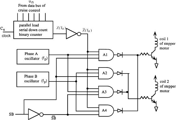
Figure 8.10 Stepper motor actuator electronics for cruise control.
The basic idea for this circuitry is to drive the stepper motor in such a way as to advance or retard the throttle in accordance with the control signal un that is stored in memory. Just as the controller periodically updates the actuator control signal, the stepper motor driver electronics continually adjusts the throttle by an amount determined by this actuator signal. This signal is, in effect, a signed number (i.e., a positive or negative numerical value). A sign bit indicates the direction of the throttle movement (advance or retard). The numerical value determines the amount of advance or retard.
The magnitude of the actuator signal (in binary format) is loaded into a parallel load serial down-count binary counter. The direction of movement is in the form of the sign bit (SB of Figure 8.10). The stepper motor is activated by a pair of quadrature phase signals (i.e., signals that are out of phase by π/2) coming from a pair of oscillators. To advance the throttle, phase A signal is applied to coil 1 and phase B signal to coil 2. To retard the throttle these phases are each switched to the opposite coil. The amount of movement in either direction is determined by the number of cycles Np(n) of A and B, one step for each cycle.
The number of cycles of these two phases is controlled by a logical signal (Z(Ta)) in Figure 8.10. This logical signal is switched low such that ![]() is high for period Ta, enabling a pair of AND gates (from the set A1, A2, A3, and A4). The length of time that
is high for period Ta, enabling a pair of AND gates (from the set A1, A2, A3, and A4). The length of time that ![]() is switched high (Ta) determines the number of cycles and corresponds to the number of steps of the motor.
is switched high (Ta) determines the number of cycles and corresponds to the number of steps of the motor.
The logical variable Z corresponds to the contents of the binary counter being zero. As long as the logical inverse of ![]() (i.e.,
(i.e., ![]() ) is high, a pair of AND gates (A1 and A3, or A2 and A4) is enabled, permitting phase A and phase B signals to be sent to the stepper motor. The pair of gates enabled is determined by the sign bit. When the sign bit is high, A1 and A2 are enabled and the stepper motor advances the throttle position as long as Z is not high. Similarly, when the sign bit is low, A3 and A4 are enabled and the stepper motor retards the throttle position. The diodes in the AND gate outputs isolate the inactive from the active AND gates.
) is high, a pair of AND gates (A1 and A3, or A2 and A4) is enabled, permitting phase A and phase B signals to be sent to the stepper motor. The pair of gates enabled is determined by the sign bit. When the sign bit is high, A1 and A2 are enabled and the stepper motor advances the throttle position as long as Z is not high. Similarly, when the sign bit is low, A3 and A4 are enabled and the stepper motor retards the throttle position. The diodes in the AND gate outputs isolate the inactive from the active AND gates.
To control the number of steps, the controller loads a binary value into the binary counter. With the contents not being zero, the appropriate pair of AND gates is enabled. When loaded with data, the binary counter counts down at the frequency of a clock (CK in Figure 8.10). When the countdown reaches zero, logical variable Z switches high (and ![]() switches low) and the gates are disabled and the stepper motor stops moving.
switches low) and the gates are disabled and the stepper motor stops moving.
The time required to count down to zero is determined by the numerical value loaded into the binary counter. By loading signed binary numbers into the binary counter, the cruise controller regulates the amount and direction of movement of the stepper motor and thereby the corresponding movement of the throttle.
Vacuum-Operated Actuator
The driver electronics for a cruise control based on a vacuum-operated system generates a variable-duty-cycle signal as described above. In this type of system, the duty cycle at any time is proportional to the control signal as explained above. For example, if at any given instant a large positive error exists between the command and actual signal, then a relatively large control signal will be generated. This control signal will cause the driver electronics to produce a large duty-cycle signal to operate the solenoid so that most of the time the actuator cylinder chamber is nearly at manifold vacuum level. Consequently, the piston will move against the restoring spring and cause the throttle opening to increase. As a result, the engine will produce more power and will accelerate the vehicle until its speed matches the command speed.
It should be emphasized that, regardless of the actuator type used, a microprocessor-based cruise control system will:
2. Measure actual vehicle speed.
3. Compute an error (error = command − actual).
4. Compute a control signal using P, PI, or PID control law.
5. Send the control signal to the driver electronics.
6. Cause driver electronics to send a signal to the throttle actuator such that the error will be reduced.
Although analog electronics are obsolete in contemporary vehicles, we include the following example of a pure analog system to illustrate principles introduced in Chapter 3 and because there remain some older vehicles with such systems on the road. A pure analog speed sensor in the form of a d-c generator is assumed. Its output voltage Vo is linearly proportional to vehicle speed ![]() :
:
![]() (37)
(37)
where Kg is the constant for the sensor.
An example of electronics for a cruise control system that is basically analog is shown in Figure 8.11.
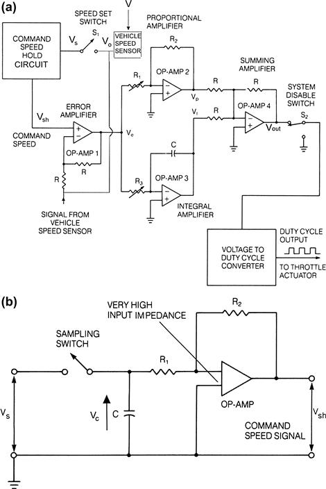
Figure 8.11 Analog cruise control configuration.
The vehicle speed sensor of Figure 8.11a generates the output Vo which is sent to the driver-operated switch for setting a voltage corresponding to desired speed (Vd) in a hold circuit such as was described in Chapter 3. This voltage value will remain until reset by the driver to a new value. The sensor voltage also provides the feedback signal to the error amplifier of this PI control system. Notice that the system uses four operational amplifiers (op amps) as described in Chapter 3 and that each op amp is used for a specific purpose. Op amp 1 is used as an error amplifier. The output of op amp 1 (Ve) is proportional to the difference between the command speed and the actual speed. The error signal is then used as an input to op amps 2 and 3. Op amp 2 is a proportional amplifier with a gain of KP = −R2/R1. Notice that R1 is variable so that the proportional amplifier gain can be adjusted. Op amp 3 is an integrator with a gain of KI = −1/R3C, which generates output voltage VI, which is given by
![]() (38)
(38)
The outputs of the proportional and integral amplifiers are added using a summing amplifier, op amp 4. The summing amplifier adds voltages VP and VI and inverts the resulting sum. The inversion is necessary because both the proportional and integral amplifiers invert their input signals while providing amplification. Inverting the sum restores the correct sense, or polarity, to the control signal.
The summing amplifier op amp produces an analog voltage, Vout, that must be converted to a duty-cycle signal before it can drive the throttle actuator. A voltage-to-duty-cycle converter is used whose output directly drives the throttle actuator solenoid. The voltage-to-duty-cycle converter is a voltage-controlled oscillator which generates an output wave form at frequency fp with duty cycle which is proportional to Vout.
Two switches, S1 and S2, are shown in Figure 8.11a. Switch S1 is operated by the driver to set the desired speed. It signals the sample-and-hold electronics (Figure 8.11b) to sample the present vehicle speed at the time S1 is activated and hold that value until the next switch operation by the driver. Voltage Vc, representing the vehicle speed at which the driver wishes to set the cruise controller, is sampled and it charges capacitor C. A very high input impedance amplifier detects the voltage on the capacitor without causing the charge on the capacitor to “leak” off. The output from this amplifier is a voltage, Vsh, proportional to the command speed that is sent to the error amplifier:
![]() (39)
(39)
where ta is the time driver activating S1.
Switch S2 (Figure 8.11a) is used to disable the speed controller by interrupting the control signal to the throttle actuator. Switch S2 disables the system whenever the ignition is turned off, the controller is turned off, or the brake pedal is pressed. The controller is switched on when the driver presses the speed set switch S1.
For safety reasons, the brake turnoff is often performed in two ways. As just mentioned, pressing the brake pedal turns off or disables the electronic control. In certain cruise control configurations that use a vacuum-operated throttle actuator, the brake pedal also mechanically opens a separate valve that is located in a hose connected to the throttle actuator cylinder. When the valve is opened by depression of the brake pedal, it allows outside air to flow into the throttle actuator cylinder so that the throttle plate is rapidly closed. The valve is shut off whenever the brake pedal is in its inactive position. This ensures a fast and complete shutdown of the speed control system whenever the driver presses the brake pedal.
Advanced Cruise Control
The cruise control system previously described is adequate for maintaining constant speed, provided that any required deceleration can be achieved by a throttle reduction (i.e. reduced engine power). The engine has limited braking capability with a closed throttle, and this braking in combination with aerodynamic drag and tire-rolling resistance may not provide sufficient deceleration to maintain the set speed. For example, a car entering a long, relatively steep downgrade in a mountainous region may accelerate due to gravity even with the throttle closed.
For this driving condition, vehicle speed can be maintained only by application of the brakes. For cars equipped with a conventional cruise control system, the driver has to apply braking to hold speed.
An advanced cruise control (ACC) system has a means of automatic brake application whenever deceleration with throttle input alone is inadequate. A somewhat simplified block diagram of an ACC is shown in Figure 8.12, emphasizing the automatic braking portion.
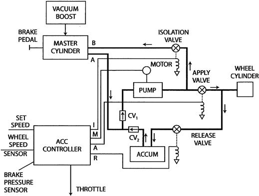
Figure 8.12 ACC system configuration.
This system consists of a conventional brake system with master cylinder wheel cylinders, vacuum boost (power brakes), and various brake lines. Figure 8.12 shows only a single-wheel cylinder, although there are four in actual practice. In addition, proportioning valves are present to regulate the front/rear brake force ratio.
In normal driving, the system functions like a conventional brake system. As the driver applies braking force through the brake pedal to the master cylinder, brake fluid (under pressure) flows out of port A and through a brake line to the junction of check valves CV1 and CV2. Check valve CV2 blocks brake fluid, whereas CV1 permits flow through a pump assembly P and then through the apply valve (which is open) to the wheel cylinder(s), thereby applying brakes.
In cruise control mode, the ACC controller regulates the throttle (as explained above for a conventional cruise control) as well as the brake system via electrical output signals and in response to inputs, including the vehicle speed sensor and set cruise speed switch. The ACC system functions as described above until the maximum available deceleration with closed throttle is inadequate. Whenever there is greater deceleration than this maximum value, the ACC applies brakes automatically. In this automatic brake mode, an electrical signal is sent from the M (i.e. motor) output of the controller to the motor, causing the pump to send more brake fluid (under pressure) through the apply valve (maintained open) to the wheel cylinder. At the same time, the release valve remains closed such that brakes are applied.
The braking pressure can be regulated by varying the isolation valve, thereby bleeding some brake fluid back to the master cylinder. By activating isolation valves separately to the four wheels, brake proportioning can be achieved. Brake release can be accomplished by sending signals from the ACC to close the apply valve and open the release valve. We present next a continuous time model for the ACC.
The vehicle model under ACC mode is given by
![]() (40)
(40)
where Tbo is the engine torque at closed throttle and TB the braking torque.
This braking torque is normally zero under steady cruise. It is only increased from zero in the ACC mode when required to maintain cruise speed.
Under normal circumstances, for a sufficiently steep downgrade (i.e. θ < 0), Tbo is negligible. For simplification purposes, it is assumed that the braking torque is linearly proportional to brake pressure pB:
![]() (41)
(41)
where KB is a constant for the brake configuration. A linearized model for the vehicle traveling on a straight road with vehicle speed ![]() is given by
is given by
![]() (42)
(42)
where KA is the brake pressure actuator constant Vd is the cruise speed set point, and u the ACC control signal.
If a PI control law is assumed for this ACC automatic braking mode, the control signal is given by
![]() (43)
(43)
where
Substituting the control signal model into the linearized vehicle mode and taking the Laplace transform of the resulting equation yield the following:
![]() (44)
(44)
Solving for δV(s) yields
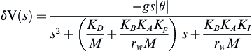 (45)
(45)
Note the similarity to the model for cruise control developed earlier in which the actuator drives the throttle plate angle. In the above equation, the negative sign of the θ for g downgrade is accounted for by replacing −θ with ![]() . The dynamic response of a car with ACC traveling along a straight horizontal road and encountering a steep downgrade (with slope
. The dynamic response of a car with ACC traveling along a straight horizontal road and encountering a steep downgrade (with slope ![]() ) is similar to that for an ordinary cruise control encountering a sudden change in slope except that the speed initially increases and then comes to an asymptotic value.
) is similar to that for an ordinary cruise control encountering a sudden change in slope except that the speed initially increases and then comes to an asymptotic value.
A simulation of this ACC was run for the same vehicle parameters of the earlier example. Here it is assumed that the vehicle encounters the steep downgrade at t = 2 s. It is further assumed for simplicity that the ACC switches instantly to automatic braking mode (when the throttle closed switch signals the controller). Figure 8.13 is a plot of vehicle speed for P-only control as well as PI control. The same coefficients are assumed for the controller and KB is taken to be four.
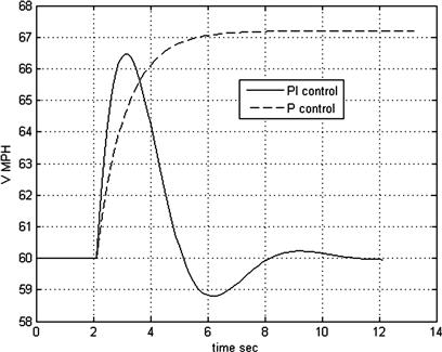
Figure 8.13 Vehicle speed with ACC on hill with long downgrade.
Figure 8.13 is a plot of the ACC speed response to a long steep downgrade of –7% encountered at t = 2 s for a vehicle with ACC that is initially in a steady 60 MPH cruise. Note that for P-only control, the speed increases to an asymptotic value of about 67 MPH. During the asymptotic range, this speed is maintained with a steady brake pressure. However, for PI control, the speed initially increases, then with applied brakes decreases with small undershoot reaching the desired cruise speed of 60 MPH. The action of various control laws was described in Chapter 1. The present simulation confirms the predicted behavior.
Another potential application for automatic braking involves separate brake pressure applied individually to all four wheels. This independent brake application can be employed for improved handling when both braking and steering are active (e.g. braking on curves). Later in this chapter, an application of automatic braking to enhance the lateral stability of the vehicle is discussed.
Antilock Braking System
One of the most readily accepted applications of electronics in automobiles has been the antilock brake system (ABS). ABS is a safety-related feature that assists the driver in deceleration of the vehicle in poor or marginal braking conditions (e.g. wet or icy roads). In such conditions, panic braking by the driver (in non-ABS-equipped cars) results in reduced braking effectiveness and, typically, loss of directional control due to the tendency of the wheels to lock (i.e. to stop rolling and to be held firmly against rotation by the brakes).
In ABS-equipped cars, the wheel is prevented from locking by a mechanism that automatically regulates the force applied to the wheels by the brakes to an optimum for any given low-friction condition. The physical configuration for an ABS is shown in Figure 8.14. In addition to the normal brake components, including brake pedal, master cylinder, vacuum boost, wheel cylinders, calipers/disks, and brake lines, this system has a set of angular speed sensors at each wheel, an electronic control module, and a hydraulic brake pressure modulator (regulator). For simplicity in the drawing, only a pair of brake pressure modulators are shown. However, in practice there is a separate modulator for each brake.
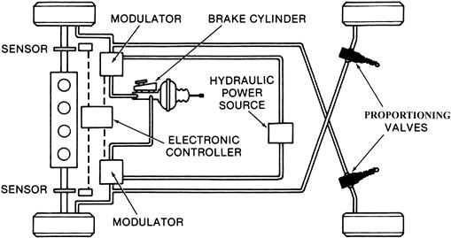
Figure 8.14 Antilock braking system.
In order to understand the ABS operation, it is first necessary to understand the physical mechanism of wheel lock and vehicle skid that can occur during braking. The car is traveling at a speed U and the wheels are rotating at an angular speed ωw where
![]() (46)
(46)
and where RPMw is the RPM of the wheel in revolutions per minute. When the wheel is rolling (no applied brakes),
![]() (47)
(47)
where rw is the tire effective radius.
When the brake pedal is depressed, the pads are forced by hydraulic pressure against the disk, as depicted schematically in Figure 8.15a. Figure 8.15b illustrates the forces applied to the wheel by the road during braking. This pressure causes a force which acts as a torque Tb in opposition to the wheel rotation. The actual force that decelerates the car is shown as Fb in Figure 8.15b. The lateral force that maintains directional control of the car is shown as FL in Figure 8.15b.
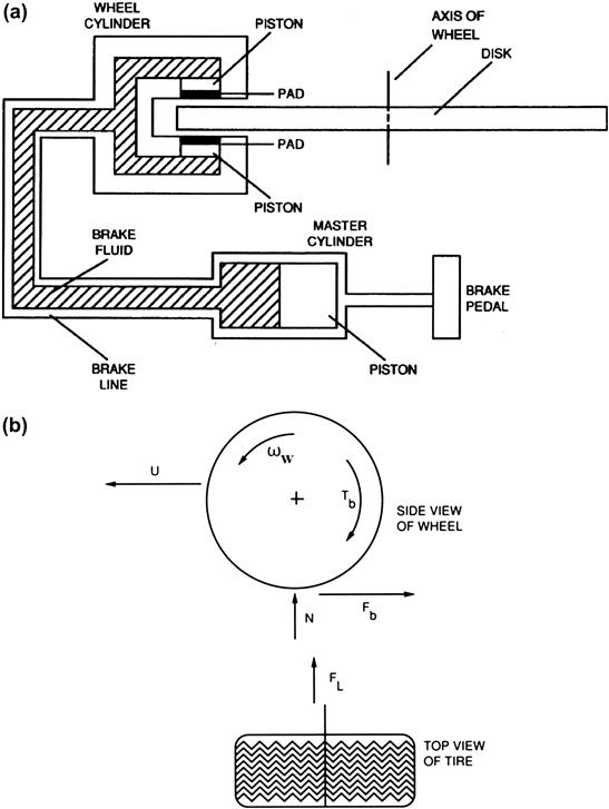
Figure 8.15 Brake configuration and forces acting on wheel.
The wheel angular speed begins to decrease, causing a difference between the vehicle speed U and the tire speed over the road (i.e. ωwrw). In effect, the tire slips relative to the road surface. The amount of slip s determines the braking force and lateral force. The slip, as a percentage of car speed, is given by
![]()
Note: A rolling tire has slip s = 0, and a fully locked tire has s = 1.
The braking and lateral forces are proportional to the normal force (from the weight of the car and from inertial forces due to deceleration) acting on the tire/road interface (N in Figure 8.15b) and the friction coefficients for braking force (Fb) and lateral force (FL):
![]() (48)
(48)
where μb is the braking friction coefficient and μL is the lateral friction coefficient.
These coefficients depend markedly on slip, as shown qualitatively in Figure 8.16. The solid curves are for a dry road and the dashed curves for a wet or icy road. As brake pedal force is increased from zero, slip increases from zero. For increasing slip, μb increases to s = so. Further increase in slip actually decreases μb, thereby reducing braking effectiveness.

Figure 8.16 Exemplary variation in friction coefficients with slip.
On the other hand, μL decreases steadily with increasing s such that for fully locked wheels the lateral force has its lowest value. For wet or icy roads, μL at s = 1 is so low that the lateral force often is insufficient to maintain directional control of the vehicle. However, directional control can often be maintained even in poor braking conditions if slip is optimally controlled. This is essentially the function of the ABS, which performs an operation equivalent to pumping the brakes (as done by experienced drivers before the development of ABS). In ABS-equipped cars under marginal or poor braking conditions, the driver simply applies a steady brake force and the system adjusts tire slip dynamically to achieve near optimum value (on average) automatically.
In an exemplary ABS configuration, control over slip is affected by regulating the brake line pressure under electronic control. The configuration for ABS is shown in Figure 8.14. This ABS regulates or modulates brake pressure to maintain slip as near to optimum for as much time as possible (e.g. at so in Figure 8.16). The operation of this ABS is based on estimating the torque Tw applied to the wheel at the road surface by the braking force Fb:
![]() (49)
(49)
The braking torque Tb is applied to the disk by the brake pads in response to brake pressure pb and is a function of pb:
![]() (50)
(50)
Although it is not necessary for ABS application, it is convenient to simplify the model for Tb to the following:
![]() (51)
(51)
where kb is a constant for the given brakes.
The difference between these two torques acts to decelerate the wheel. In accordance with basic Newtonian mechanics, the wheel torque Tw is related to braking torque and wheel deceleration by the following equation:
![]()
where Iw is the wheel moment of inertia about its rotational axis and ![]() is the wheel deceleration
is the wheel deceleration ![]() , that is, the rate of change of wheel speed.
, that is, the rate of change of wheel speed.
During heavy braking under marginal conditions, sufficient braking force is applied to cause wheel lock-up (in the absence of ABS control). We assume such heavy braking for the following discussion of the ABS. As brake pressure is applied, Tb increases and ωw decreases, causing slip to increase. The wheel torque is proportional to μb, which reaches a peak at slip so. Consequently, the wheel torque reaches a maximum value (assuming sufficient brake force is applied) at this level of slip and decreases for s > so. For this region of slip, the slope of μb is negative (i.e. ![]() ) and wheel deceleration is unstable causing ωw → 0 resulting in wheel lock condition. It is the function of the ABS to regulate Tb to maintain slip near optimum as explained below.
) and wheel deceleration is unstable causing ωw → 0 resulting in wheel lock condition. It is the function of the ABS to regulate Tb to maintain slip near optimum as explained below.
Figure 8.17 is a sketch of wheel torque versus slip during ABS action illustrating the peak Tw. After the peak wheel torque is sensed electronically, the electronic control system commands that brake pressure be reduced (via the brake pressure modulator). This point is indicated in Figure 8.17 as the limit point of slip for the ABS. As the brake pressure is reduced, slip is reduced and the wheel torque again passes through a maximum.
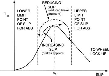
Figure 8.17 Wheel torque vs. slip under ABS action.
The wheel torque reaches a value below the peak on the low slip side denoted lower limit point of slip and at this point brake pressure is again increased. The system will continue to cycle, maintaining slip near the optimal value as long as the brakes are applied and the braking conditions lead to wheel lock-up.
The ABS control laws and algorithms are, naturally, proprietary for each manufacturer. Rather than dealing with such proprietary issues here, an ABS control concept is presented here based upon a paper by the author of this book and which has demonstrated successful ABS operation in laboratory (wheel dynamometer) tests. This discussion can be considered exemplary of much of the mechanical dynamics as well as control algorithms.
An ideal ABS control would maintain braking force/torque such that slip would remain at exactly the optimum slip (i.e. so) for any given tire/road condition. However, a suboptimal control system having very near optimal performance can be achieved by cycling brake pressure such that slip cycles up and down about the optimum as depicted qualitatively in Figure 8.17. The cycling should be such that the average of the time varying s and μb, μL are very close to optimum.
The present exemplary ABS control is based upon the use of a so-called sliding mode observer (SMO). The SMO is a robust state vector estimator that has the capability of estimating very closely the state vector of a dynamic system (see Chapter 1 for the definition of a state vector). The SMO for the present discussion estimates a single-dimensional state vector, the differential torque applied to the wheel, (δTb), where
![]() (53)
(53)
Rewriting Eqn (53) yields a form from which the SMO can be readily derived:
![]() (54)
(54)
The goal for the SMO for this application is to calculate an estimate ![]() of the differential torque. It obtains
of the differential torque. It obtains ![]() by solving the following differential equation for the estimate
by solving the following differential equation for the estimate ![]() of wheel angular speed:
of wheel angular speed:
![]() (55)
(55)
Where m is the SMO gain that must satisfy the following inequality:
![]() (56)
(56)
The SMO requires an accurate, precise measurement of wheel angular speed (ωw). The desired estimate ![]() is the solution to the following first-order differential equation:
is the solution to the following first-order differential equation:
![]() (57)
(57)
Effectively, ![]() is a first-order low-pass-filtered version of the right-hand side of the above equation. The low-pass filter (LPF) bandwidth (i.e. 1/τ) must be sufficiently large to accommodate the relatively large fluctuations in wheel angular speed. It is possible to use a higher-order than first-order low-pass filter. Experiments and simulations have been run with 2nd-order LPF with good braking performance. The SMO generates a very close estimate of δTb such that the control logic can detect that extremal values for the actual differential torque have occurred by detecting extremal values of the SMO estimate
is a first-order low-pass-filtered version of the right-hand side of the above equation. The low-pass filter (LPF) bandwidth (i.e. 1/τ) must be sufficiently large to accommodate the relatively large fluctuations in wheel angular speed. It is possible to use a higher-order than first-order low-pass filter. Experiments and simulations have been run with 2nd-order LPF with good braking performance. The SMO generates a very close estimate of δTb such that the control logic can detect that extremal values for the actual differential torque have occurred by detecting extremal values of the SMO estimate ![]() . This estimate is the input to the control algorithm for regulating brake pressure.
. This estimate is the input to the control algorithm for regulating brake pressure.
The actual control algorithm for applying or releasing brakes is based upon the estimate of δTb. Whenever the slip passes the optimal value (so), either increasing or decreasing the ![]() has an extremal value. One control scheme incorporates an extremal value detector applied to
has an extremal value. One control scheme incorporates an extremal value detector applied to ![]() . Whenever an extremum is detected with brakes applied, this indicates s has crossed so while increasing. Upon detection of this extremum, the control generates a command signal to release brake pressure (using a mechanism described below). Conversely, whenever an extremal value of
. Whenever an extremum is detected with brakes applied, this indicates s has crossed so while increasing. Upon detection of this extremum, the control generates a command signal to release brake pressure (using a mechanism described below). Conversely, whenever an extremal value of ![]() is detected with brakes not being applied (or at reduced brake pressure), this indicates that s has crossed so while decreasing. Upon detecting this condition, the control system generates a signal that causes brake pressure to be reapplied.
is detected with brakes not being applied (or at reduced brake pressure), this indicates that s has crossed so while decreasing. Upon detecting this condition, the control system generates a signal that causes brake pressure to be reapplied.
During ABS operation, the control logic essentially detects that slip has increased beyond so, and at some point between so and the upper limit point of slip for ABS (as shown in Figure 8.17), this logic detects an impending wheel lock condition and generates control signals that cause brake pressure to rapidly decrease. With brake pressure reduced, the wheel tends toward a rolling condition and slip decreases as depicted in Figure 8.17. As the slip crosses so while decreasing, μb increases to its maximum value at so and then decreases. The corresponding δTb has an extremum as s crosses so. The SMO detects the extremal value of ![]() , thereby creating a logic condition that brakes are to be re-applied.
, thereby creating a logic condition that brakes are to be re-applied.
In an actual ABS, the brakes are individually controlled at each wheel. Separate control of each wheel is required because during braking, the inertial forces can result in different normal force (N) at each wheel. In addition, the friction coefficient may well be different for each tire/road interface.
There are two major benefits to ABS. One of these is achieving optimal friction coefficient at each wheel. The other is to maintain sufficient lateral friction coefficient (μL) for good directional control of the vehicle during stopping.
The mechanism for modulating brake pressure is illustrated in Figure 8.18.

Figure 8.18 Schematic illustration of ABS.
In Figure 8.18 the notation is as follows:
| BP | Brake pedal |
| MC | Master cylinder |
| K | Brake fluid reservoir |
| BV | Blocking valve |
| DV | Pressure dump valve |
| RV | Repressurization valve |
| P | Pump |
| A | Accumulator |
| S | Wheel speed sensor |
| WC | Wheel cylinder |
| V1,V2,V3 | Actuator control signals. |
During braking with ABS control, the driver is assumed to apply brake pressure to the line connecting MC and WC. The driver is assumed to maintain a relatively high pressure. Although Figure 8.18 depicts ABS for a single wheel, it is assumed that a separate set of valves are supplied for each of the four wheel cylinders.
Each of the valves depicted in Figure 8.18 are two-position solenoid-operated valves, each having two separate functions. The blocking valve in the inactive position for V1 = 0 passes brake fluid under pressure from its input line to its output line. Under normal (non-ABS) braking, the dump valve (V2 = 0) passes this fluid from its input to its output line which leads to the repressurization valve. This latter valve passes the pressurized brake fluid to the wheel cylinder which thereby applies brake torque to the corresponding wheel.
Whenever the ABS control detects a potential wheel lock-up owing to slip s > so (due to the negative dμb/ds), it generates nonzero control signals V1, V2, and V3 in a precise sequence. In the exemplary ABS, potential wheel lock is detected by an extremum in ![]() with brakes applied. The control sends a voltage V1 to BV which causes it to switch to a brake pressure-blocked position. In this position the master cylinder is isolated from the wheel cylinder by the BV. Only the input line to BV is under driver-applied brake pressure. A few milliseconds after the BV is activated, the control generates a voltage V2 that activates the DV which switches it to its second position. In this position the line to the RV and wheel cylinder are connected to the reservoir and the WC pressure drops rapidly toward 0.
with brakes applied. The control sends a voltage V1 to BV which causes it to switch to a brake pressure-blocked position. In this position the master cylinder is isolated from the wheel cylinder by the BV. Only the input line to BV is under driver-applied brake pressure. A few milliseconds after the BV is activated, the control generates a voltage V2 that activates the DV which switches it to its second position. In this position the line to the RV and wheel cylinder are connected to the reservoir and the WC pressure drops rapidly toward 0.
During all times a pump (P) maintains a supply of brake fluid under pressure in accumulator A. In its deactivated state (i.e. V3 = 0), the RV isolates the accumulator from the line leading to the WC and provides a stop in the A output line. This A pressure is the pressure that is used to repressure the WC at the appropriate time. This appropriate time is the time at which the control system detects an extremum in ![]() for brakes “off” (or low Tb). When the controller detects this condition, it initially sets control voltage V2 = 0, thereby deactivating DV. A few milliseconds after V2 is set to zero, the controller generates voltage V3 that activates the repressurization valve. When activated, the RV connects the A with its pressurized brake fluid to the WC. It simultaneously applies the pressure to the output line of the DV which also pressurizes the BV output line. The pressurized WC applies the force required to apply brake torque Tb to the wheel.
for brakes “off” (or low Tb). When the controller detects this condition, it initially sets control voltage V2 = 0, thereby deactivating DV. A few milliseconds after V2 is set to zero, the controller generates voltage V3 that activates the repressurization valve. When activated, the RV connects the A with its pressurized brake fluid to the WC. It simultaneously applies the pressure to the output line of the DV which also pressurizes the BV output line. The pressurized WC applies the force required to apply brake torque Tb to the wheel.
Assuming that a low μb condition is maintained, the process of increasing slip with s passing so and a new extremal valve in ![]() is detected. The entire process of pressure dump followed by represurization is repeated. The cycling of the ABS normally continues until the wheel speed with brakes “off” is below a pre-set value (e.g. 1–5 MPH) or until the driver releases the brake pedals.
is detected. The entire process of pressure dump followed by represurization is repeated. The cycling of the ABS normally continues until the wheel speed with brakes “off” is below a pre-set value (e.g. 1–5 MPH) or until the driver releases the brake pedals.
Figure 8.19 illustrates the braking during an ABS action in simulation of an experimental system. In this illustration, the vehicle is initially traveling at 55 mph and the brakes are applied as indicated by decreasing speed of Figure 8.19a. The solid curve of Figure 8.19a depicts vehicle speed over the ground and the dashed curve the instantaneous wheel speed (rwωw). The wheel speed begins to drop until the control detects incipient wheel lock (e.g. for an extremum of ![]() ). At this point, the ABS reduces brake pressure and the wheel speed increases until the control reaches the condition to reapply brake pressure. With the high applied brake pressure, the wheels again tend toward lock-up and ABS reduces brake pressure. The cycle continues until the vehicle is slowed sufficiently.
). At this point, the ABS reduces brake pressure and the wheel speed increases until the control reaches the condition to reapply brake pressure. With the high applied brake pressure, the wheels again tend toward lock-up and ABS reduces brake pressure. The cycle continues until the vehicle is slowed sufficiently.
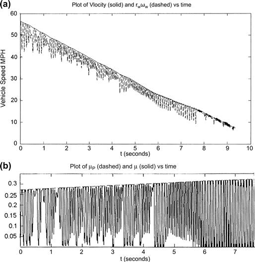
Figure 8.19 Illustration of ABS action.
Figure 8.19b depicts the instantaneous friction coefficient μb(t). It can be seen that the ABS action of releasing and then reapplying brake pressure causes this μb to cycle back and forth about its peak value (μb(so)). Similar results to those of Figure 8.19 were achieved in laboratory tests with suitable instrumentation.
It should be noted that by maintaining slip near so, the maximum deceleration is achieved for a given set of conditions. Some reduction in lateral force occurs from its maximum value by maintaining slip near so. However, in most cases the lateral force is large enough to maintain directional control, thereby permitting the driver to steer the vehicle.
In some antilock brake systems, the mean value of the slip oscillations is shifted below so, sacrificing some braking effectiveness to enhance directional control. This can be accomplished by adjusting the upper and lower slip limits.
Tire-Slip Controller
Another benefit of the ABS is that the brake pressure modulator can be used for ACC as explained earlier as well as for tire-slip control. Tire slip is effective in moving the car forward just as it is in braking. Under normal driving circumstances with powertrain torque applied to the drive wheels, the slip that was defined previously for braking is negative. That is, the tire is actually moving at a speed that is greater than for a purely rolling tire (i.e. rwωw > U). In fact, the traction force is proportional to slip.
For wet or icy roads, the friction coefficient can become very low and excessive slip can develop. In extreme cases, one of the driving wheels may be on ice or in snow while the other is on a dry (or drier) surface. Because of the action of the differential (see Chapter 7 and Figure 7.26), the low-friction tire will spin and relatively little torque will be applied to the dry-wheel side. In such circumstances, it may be difficult for the driver to move the car even though one wheel is on a relatively good friction surface.
The difficulty can be overcome by applying a braking force to the free spinning wheel. In this case, the differential action is such that torque is applied to the relatively dry-wheel surface and the car can be moved. In the example ABS, such braking force can be applied to the free spinning wheel by the hydraulic brake pressure modulator (assuming a separate modulator for each drive wheel). Control of this modulator is based on measurements of the speed of the two drive wheels. Of course, the ABS already incorporates wheel speed measurements, as discussed previously. The ABS electronics have the capability of performing comparisons of these two wheel speeds and of determining that braking is required of one drive wheel to prevent wheel spin.
Antilock braking can also be achieved with electrohydraulic brakes. An electrohydraulic brake system was described in the section of this chapter devoted to advanced cruise control (ACC).
Recall that for ACC a motor-driven pump supplied brake fluid through a solenoid-operated “brakes” apply valve to the wheel cylinder. For ACC application of the brakes, the apply and isolation valves operate separately to regulate the braking to each of the four wheels.
Electronic Suspension System
An automotive suspension system consists of springs, shock absorbers, and various linkages to connect the wheel assembly to the car body. The purpose of the suspension system is to isolate the car body motion as much as possible from wheel vertical motion due to rough road input. Figure 8.20 depicts, schematically, the suspension system for the front wheels of a front wheel drive car. In essence a suspension system is a mass, spring, damping assembly that connects the car body (whose mass is called the “sprung” mass to the wheel/axle, brake and other linkages connected to them, which are called the “unsprung” mass).
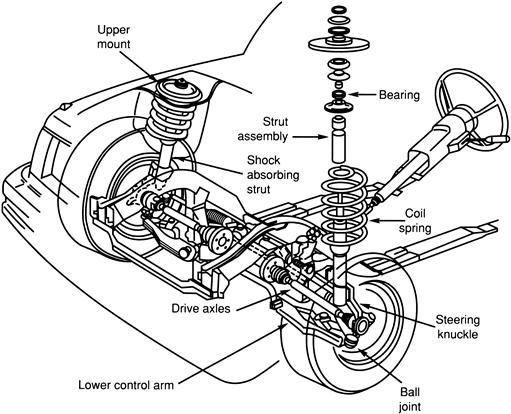
Figure 8.20 Illustration of front suspension system.
The two primary subjective performance measures from a driver/passenger standpoint are ride and handling. Ride refers to the motion of the car body in response to road bumps or irregularities. Handling refers to how well the car body responds to dynamic vehicle motion such as cornering or hard braking.
Damping in the suspension system is provided by the shock absorber portion of the strut assemble. Viscous damping is provided by fluid motion through orifices in a piston portion of the strut. The structure and details of a strut are given later in this chapter, but the interested reader can look ahead to Figure 8.23. For the present, attention is focused on the influence of strut damping on ride and handling. Generally speaking, ride is improved by lowering the shock absorber damping, whereas handling is improved by increasing this damping. In traditional suspension design, the damping parameter is fixed and is chosen to achieve a compromise between ride and handling (i.e. an intermediate value for shock absorber damping is chosen).
In electronically controlled suspension systems, this damping can be varied depending on driving conditions and road roughness characteristics. That is, the suspension system adapts to inputs to maintain the best possible ride, subject to handling constraints that are associated with safety.
There are two major classes of electronic suspension control systems: active and semi-active. The semi-active suspension system is purely dissipative (i.e. power is absorbed by the shock absorber under control of a microcontroller). In this system, the shock absorber damping is regulated to absorb the power of the wheel motion in accordance with the driving conditions.
In an active suspension system, power is added to the suspension system via a hydraulic or pneumatic power source. At the time of the writing of this book, electronic control of commercial suspension systems is primarily semi-active. In this chapter, we explain the semi-active system first, then the active one.
The primary purpose of the semi-active suspension system is to provide a good ride for as much of the time as possible without sacrificing handling. Good ride is achieved if the car’s body is isolated as much as possible from the road surface variations. The vertical input to the unsprung mass motion is the road surface profile. For a car traveling at a steady speed, this input is a random process. Depending upon the nature of the road surface (i.e. newly paved road vs. ungraded gravel dirt road), this random process may either be a stationary or a nonstationary process. For the following discussion we assume a stationary random process. A semi-active suspension controls the shock absorber damping to achieve the best possible ride without sacrificing handling performance.
In addition to providing isolation of the sprung mass (i.e. car body and contents), the suspension system has another major function. It must also dynamically maintain the tire normal force as the unsprung mass (wheel assembly) travels up and down due to road roughness. Recall from the discussion of antilock braking that braking and lateral forces depend on normal tire force. Of course, in the long-term time average, the normal forces will total the vehicle weight plus any inertial forces due to acceleration, deceleration, or cornering.
However, as the car travels over the road, the unsprung mass moves up and down in response to road input. This motion causes a variation in normal force, with a corresponding variation in potential cornering or braking forces. For example, while driving on a rough curved road, there is a potential loss of steering or braking effectiveness if the suspension system does not have good damping characteristics. We consider next certain aspects of vehicle dynamics to understand the role played by electronically controlled suspension.
The geometry for describing the vehicle motion relative to the suspension is depicted in Figure 8.21a and b. In this figure, three major axes are defined for the vehicle: 1) longitudinal; 2) lateral and 3) vertical. The ECEF inertial coordinate system axes are denoted (x′,y′,z′). The vehicle body axes are denoted (x,y,z).

Figure 8.21 Schematic illustration of suspension.
The longitudinal axis is a line in the plane of symmetry through the center of gravity (CG) parallel to a ground reference plane. The ground plane is the plane through the wheel axles when the vehicle is sitting on an exactly horizontal plane. In this configuration, the deflection of the front and rear springs due to vehicle weight depends upon the location of the CG along the longitudinal axis.
Figure 8.21 is a side view of the vehicle depicting the body longitudinal axis x (fixed to the vehicle). This figure also depicts the x axis for the vehicle at rest with the x′ axis which constitutes an inertial (e.g., ECEF) reference. In this figure, the x axis is deflected by a “pitch angle” αp relative to the x′ axis. The vertical displacement of the CG is denoted δzcg in the figure and is called heave. The front and rear springs are assumed to be identical right and left. The front suspension spring rate is denoted KF and the rear KR. Viscous damping is also assumed to be symmetrical right and left and has linear damping coefficients DF and DR for front and rear respectively (in the present, simplified model).
Figure 8.21b depicts the vehicle in a front view for which the body lateral axis (y) is shown in the rest position by the dashed line y′ and in the deflected position by the solid line. The angle ![]() is the “roll” angle about the longitudinal axis. The z axis is orthogonal to the x,y plane through the CG. The y′ and z′ axis are part of the inertial reference for the following discussion on vehicle dynamic motion.
is the “roll” angle about the longitudinal axis. The z axis is orthogonal to the x,y plane through the CG. The y′ and z′ axis are part of the inertial reference for the following discussion on vehicle dynamic motion.
It is beyond the scope of this book to present a full discussion of vehicle dynamics which involves sets of coupled nonlinear differential equation models. Rather, the goal here is to focus on electronic control of the suspension and to illustrate the corresponding aspect of vehicle dynamics for a few representative maneuvers. For this purpose a set of simplified linear dynamic models are presented. In such simplified models there are many forces acting on the vehicle sprung mass including: drivetrain and braking torques/forces, inertial forces, and the normal forces coupled from the unsprung mass acting on the tires to the sprung mass.
The normal forces acting on the tires are different for all four wheels whenever the vehicle is maneuvering. These forces include components due to the vehicle weight as well as reaction forces to inertial forces due to vehicle dynamics. These four forces have the following notations:

We begin with a relatively simple example vehicle maneuver consisting of braking on a straight and level road. The front and rear forces acting on the car from the tires are denoted FF and FR respectively. These forces are positive for acceleration and negative for braking, which is assumed here, and are given by
![]() (58)
(58)
where μF is the friction coefficient for front tires and μR is the friction coefficient for rear tires.
The combination of these braking forces produces a moment about the CG Tb given by
![]() (59)
(59)
Countering this moment is a moment (Tn) about the CG due to the tire normal forces given by
![]()
where
![]() (60)
(60)
and where a and b are the distances along the longitudinal axis of the vehicle from the CG to the front and rear axles respectively (i.e. see Figure 8.21a).
The normal forces acting on the tires are transmitted through the tires to the spring/damper system of the suspension. For the present, the tire dynamics are neglected although they are included in a later example. The forces NF and NR produce a deflection in the suspension springs from the unloaded positions such that ![]() and
and ![]() are given by:
are given by:
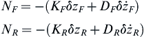 (61)
(61)
where δzF is the deflection of front spring and δzR the deflection of rear spring.
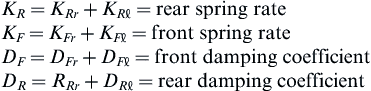 (62)
(62)
Note that in the absence of any vertical motion of the CG (i.e. it is assumed here that ![]() ), the normal forces sum to the vehicle weight (WV):
), the normal forces sum to the vehicle weight (WV):
![]() (63)
(63)
Furthermore, it is reasonable to assume that front and rear tires have identical friction coefficient
![]()
The total force acting on the vehicle due to braking is given by
![]()
The moment acting around the CG due braking (Tb) is given by
![]()
The sum of the moments of all forces acting on the sprung mass results in an angular acceleration of the pitch angle ![]() about the lateral (y) axis, yielding the following model:
about the lateral (y) axis, yielding the following model:
![]() (64)
(64)
![]()
![]()
For sufficiently small pitch-angle changes the front and rear displacement and vertical velocity are given by:
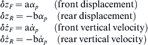 (65)
(65)
Substituting these relationships into the pitch dynamic Eqn (64) yields
![]() (66)
(66)
Simplifying and rearranging terms in this equation yield the following second-order differential equation in ![]() :
:
![]() (67)
(67)
where
![]()
The operational transfer function (Hα(s)) relating braking force to pitch angle is given by
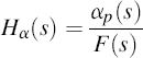
![]() (68)
(68)
where
![]()

![]()
Solution to this equation for the pitch dynamics due to an arbitrary braking force function F(t) is found using the methods of Chapter 1 or for any given vehicle via simulation. For example, the pitch-angle response to a step of amplitude change in braking force of magnitude Fo increases from αp = 0 with ![]() rising toward an asymptotic value (αpss) of
rising toward an asymptotic value (αpss) of
![]() (69)
(69)
Depending on the damping ratio ζ, there may be overshoot in αp before settling to αpss where, with the sign convention of Figure 8.21a, αpss < 0.
In addition to the operational transfer function, the pitch dynamics due to braking are given by the sinusoidal frequency response Hα(jω), which is given by
![]() (70)
(70)
The peak response occurs at ω = ωn and has magnitude
![]() (71)
(71)
and a 90° phase shift from F(jω) to αp(jω). The importance of damping in determining the resonant response of pitch dynamics is clear from this frequency response.
Recall from the discussion of ABS that the braking force during periods in which ABS is active is time varying and is often essentially periodic. The pitch dynamic response to ABS cycling is potentially a concern in ride dynamics, although the excitation frequency is normally far from pitch dynamic resonance. Nevertheless, electronically damping, as discussed later, could potentially improve ride quality.
The pitch dynamic sinusoidal frequency response (although greatly simplified) has been developed and shown to be determined by suspension spring rate and damping. A similar set of equations describe the vertical displacement (i.e. heave) dynamics. A similar sinusoidal frequency response can be derived for heave. However, this discussion is deferred to a later section in which the vertical dynamic models include wheel and tire dynamics. Later in this chapter a model is developed with these dynamics included. For the moment, we consider these dynamics and the associated frequency response qualitatively for an exemplary vehicle.
Figure 8.22 illustrates qualitatively a representative tire normal force variation as a function of frequency of excitation for a fixed-amplitude, variable-frequency sinusoidal excitation (see Chapter 1 for a discussion of sinusoidal frequency response) for an actual vehicle. The solid curve is the response for a relatively low-damping-coefficient shock absorber and the dashed curve is the response for a relatively high damping coefficient.
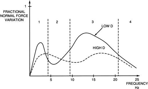
Figure 8.22 Normal force variation due to sinusoidal excitation vs. frequency.
The ordinate of the plot in Figure 8.22 is the ratio of amplitude of force variation to the average normal load (i.e. due to weight). There are two relative peaks in this response. The lower peak is approximately 1–2 Hz and is generally associated with spring/sprung mass oscillation. The second peak, which is in the general region of 12–15 Hz, is resonance of the spring/unsprung mass combination.
Generally speaking, for any given fixed suspension system, ride and handling cannot both be optimized simultaneously. A car with a good ride is one in which the sprung mass motion/acceleration due to rough road input is minimized. In particular, the sprung mass motion in the frequency region from about 2 to 8 Hz has often been found to be the most important for good subjective ride. Good ride is achieved for relatively low damping (low D in Figure 8.22).
For low damping, the unsprung mass moves relatively freely due to road input while the sprung mass motion remains relatively low. Note from Figure 8.22 that this low damping results in relatively high variation in normal force, particularly near the two peak frequencies. That is, low damping results in relatively poor handling characteristics.
With respect to the four frequency regions of Figure 8.22, the following generally desired suspension damping characteristics can be identified:
| Region | Frequency (Hz) | Damping |
| 1: Sprung mass mode | 1–2 | High |
| 2: Intermediate ride | 2–8 | Low |
| 3: Unsprung mass resonance | 8–20 | High |
| 4: Harshness | >20 | Low |
Another major input to the vehicle that affects handling is steering input that causes maneuvers out of the ECEF inertial reference vertical plane (e.g. cornering). Whenever the car is executing such maneuvers, there is a lateral acceleration. This acceleration acting through the center of gravity causes the vehicle to roll in a direction opposite to the maneuver.
Another relatively simple example of vehicle dynamics involves the vehicle encountering a curve in a level road. For convenience assume that the car is traveling a straight road for t < 0 and then encounters the curve at t = 0. This example illustrates the influence of such a maneuver on roll dynamics (i.e. ![]() ). For this example it is necessary to include the variable ψ (which was introduced earlier in the chapter and is called yaw) in the dynamic model. It is the change in direction of the vehicle longitudinal axis relative to its direction on the straight level road. Because the road for t < 0 is straight, the initial direction forms the ECEF inertial reference frame for this example. The notation for the time rate of change of ψ is r:
). For this example it is necessary to include the variable ψ (which was introduced earlier in the chapter and is called yaw) in the dynamic model. It is the change in direction of the vehicle longitudinal axis relative to its direction on the straight level road. Because the road for t < 0 is straight, the initial direction forms the ECEF inertial reference frame for this example. The notation for the time rate of change of ψ is r:
![]() (72)
(72)
Similarly, the notation for ![]() is taken to be p:
is taken to be p:
![]() (73)
(73)
The lateral velocity component of the CG is denoted v:
![]() (74)
(74)
The inertial forces due to the motion of the car along the curve create a rolling moment TR about the CG given by
![]() (75)
(75)
where uo is the vehicle speed (assumed constant) and M the vehicle mass.
The sum of the moments about the CG for this maneuver yields the following approximate differential equation:
![]() (76)
(76)
where Ixx is the moment of inertia of the sprung mass structure about the body longitudinal axis
![]()
![]() (77)
(77)
where w is the distance between right and left tire planes of symmetry (Figure 8.21a).
In this equation, a term proportional to the cross product of inertia ![]() has been neglected without serious loss of generality as it is usually small except for relatively high
has been neglected without serious loss of generality as it is usually small except for relatively high ![]() . The above equation can be rewritten in terms of the inertial (rolling) moment (TR) in the form
. The above equation can be rewritten in terms of the inertial (rolling) moment (TR) in the form
![]() (78)
(78)
where
![]()
If the curve is a segment of a constant radius circle, then during the constant turn maneuver the moment T can be given as
![]() (79)
(79)
It can be shown that for a vehicle traveling along a curve of constant radius R at a constant speed uo, T0 is given by
![]()
The operational transfer function for the roll dynamics ![]() is given by
is given by
 (80)
(80)
The dynamic response ![]() in roll to a step encounter with the curve at t = 0 has the same qualitative shape as that found for the pitch response to a step of applied brakes. The roll damping coefficient Lp which is proportional to the strut damping coefficient has the same influence on
in roll to a step encounter with the curve at t = 0 has the same qualitative shape as that found for the pitch response to a step of applied brakes. The roll damping coefficient Lp which is proportional to the strut damping coefficient has the same influence on ![]() as it does on αp(t). The steady-state roll angle
as it does on αp(t). The steady-state roll angle ![]() after the transient response has decayed is given by
after the transient response has decayed is given by
![]() (81)
(81)
That is, the suspension spring rate determines the roll for a given steady turn rate. For passenger cars under normal driving conditions, the sinusoidal frequency response in roll is typically of less interest than for pitch or heave dynamics. A sinusoidal roll moment input might come, for example, from an oscillatory steering wheel input. This is not encountered in normal passenger car operation.
Car handling generally improves if the amount of roll for any given maneuver is reduced. The rolling rate for a given car and maneuver is improved if spring rate and shock absorber damping are increased.
In Chapter 1, we discussed the dynamics of a spring/mass/damping system, identifying resonant frequency and unity damping Dc (i.e. ζ = 1):
![]()
For good ride, the damping should be as low as possible. However, from practical design considerations, the minimum damping is generally in the region of 0.1 < D/Dc < 0.2. For optimum handling, the damping is in the region of 0.6 < D/Dc < 0.8.
Technology has been developed permitting the damping characteristics of shock absorber/strut assembly to be varied electrically, which in turn permits the ride/handling characteristics to be varied while the car is in motion. For an understanding of the operation of electronic suspension control, it is helpful to review the operation of a strut (shock absorber) with reference to Figure 8.23. Physically, this strut consists of a closed cylinder with a movable piston. Opposite ends of this strut are attached to the vehicle body (sprung mass) and the wheel axle assembly (unsprung mass). The strut is filled with oil which can pass through relatively small apertures in the piston, thereby allowing relative motion between the attachment points. The strut provides viscous damping force whenever the piston is moving in the cylinder that is an increasing function of the relative piston/cylinder velocity, the size of the apertures, and the fluid viscosity. Although the force–velocity relationship is nonlinear, in the following analysis this relationship was modeled as approximately linear.

Figure 8.23 Strut physical configuration.
Under normal steady-cruise conditions, damping is electrically set low (e.g. with relatively large aperture) yielding a good ride. However, under dynamic maneuvering conditions (e.g. cornering), the damping is set high (relatively small aperture) to yield good handling. Generally speaking, as shown in the above, simplified example, high damping reduces vehicle roll in response to cornering or turning maneuvers, and it tends to maintain tire force on the road for increased cornering forces. Variable damping suspension systems can improve safety, particularly for vehicles with a relatively high center of gravity (e.g. SUVs). Before proceeding with a discussion of electronically controlled strut damping, it is necessary to include tire dynamics in our vehicle dynamic model.
The tire dynamics in the vehicle dynamic models can be introduced adequately for the purposes of reviewing electronically controlled suspension by considering a single strut configuration. This configuration and the model being developed apply to all four suspension assemblies. The model is often called “the quarter car model” (QCM). It is in effect a unicycle model. The configuration to be considered for this QCM is depicted in Figure 8.24.
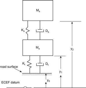
Figure 8.24 QCM car suspension configuration.
In this figure, the following notation is used:
y0 = road height above a horizontal inertial reference (e.g. ECEF)
y1 = height of unsprung mass above datum
y2 = height of sprung mass above datum
Typically, tire damping is very small in comparison with strut damping so it is assumed to be negligible here.
A pair of differential equations can be written separately by summing forces acting on the sprung mass and on the unsprung mass. For the unsprung and sprung mass, respectively, the dynamic models are given by
![]() (82)
(82)
![]() (83)
(83)
Solution of Eqn (84) can be found in two ways. The first way we consider leads to a closed-form analytical solution. Alternatively, the solution method that is best suited for numerical evaluation is to write the above equations in terms of a set of four state variable equations with state vector x given by
![]()
where
Taking the Laplace transform of Eqns (82) and (83) (with zero initial conditions) yields a pair of coupled algebraic equations in complex frequency s:
![]() (84)
(84)
![]()
In matrix form, this pair of equations can be written in the form
![]() (85)
(85)
where
![]() (86)
(86)
The two-dimensional state vector [y1, y2]T is found using matrix methods yielding
![]() (87)
(87)
The 2 × 2 matrix A is readily inverted using standard methods from matrix algebra yielding an analytical solution for y1 or y2. The time response for an arbitrary yo(t) can be found using the inverse Laplace methods of Chapter 1. However, for evaluating ride and handling, the frequency response characteristics are the most meaningful quantitative representation.
Our primary interest here is in finding the sprung mass motion since this directly affects “ride” quality. Ride is best characterized by the sprung mass acceleration (as) for any given road profile yo(x) where
![]() (88)
(88)
The operational transfer function relating as(s) to y0(s) can be shown to be given by
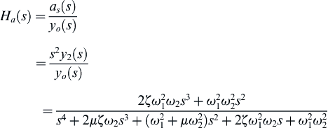 (89)
(89)
where
Handling is strongly influenced by the variation in tire normal force δN. This normal force is proportional to the relative displacement d = y0 − y1:
![]()
The transfer function HH(s) is defined as
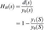 (90)
(90)
The solution for y1(s) from the matrix equation yields the following:
![]() (91)
(91)
As an illustration of the variation in relative displacement d vs. road displacement yo vs. frequency, a plot of the sinusoidal frequency response for HH(jω) is given in Figure 8.25. For this figure, a representative QCM was used with the following parameters in English units:
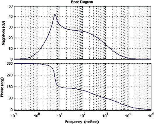
Figure 8.25 Frequency response for HH(s).
Figure 8.25 presents the magnitude of this frequency response (in dB) as 20 log |HH(jω)| and the phase of HH(jω) vs. log(ω). It can be seen that this QCM has a relatively sharp resonance at ![]() rad/s or about 1.1 Hz. This resonance is primarily due to the dynamic response of the unsprung mass.
rad/s or about 1.1 Hz. This resonance is primarily due to the dynamic response of the unsprung mass.
In evaluating the influence of suspension system parameters on ride and handling, the road profile must be modeled. It is widely known that the road profile is a random process. A random process is quantitatively represented by its amplitude and spectral statistics. The amplitude statistics are given by its probability distribution function Py(Y) = p(y ≤ Y). Its spectral statistics are represented by the power spectral density for yo which is denoted Wo(f) and is given by
![]() (92)
(92)
where
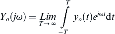 (93)
(93)
However, road profiles are functions of distance along the road surface (i.e. yo(x)). This road profile random process can be converted to a time function by considering motion at a constant speed uo where
![]()
The time function yo(t) is given by
![]()
The International Standards Organization (ISO) has established a standard model for Wo(f), which is roughly an inverse function of frequency f.
Ride is best characterized quantitatively by the RMS (root-mean-squared) value of the sprung mass acceleration ![]() :
:
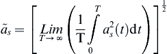
This RMS value can also be found from the power spectral density (Wa(f)) for as. Assuming that the road profile is a stationary random process (or a quasi-stationary process, i.e. stationary over large segments), the RMS value for as is given by
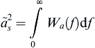
For a stationary random process, the power spectral density Wa(f) is given by
![]() (94)
(94)
Thus, the ride quality can be represented by the integral
 (95)
(95)
The above equation for ![]() illustrates the significance of the sinusoidal frequency response of the sprung mass to road excitation. The important suspension parameters in Ha(jω) are the sprung and unsprung mass as well as their ratio
illustrates the significance of the sinusoidal frequency response of the sprung mass to road excitation. The important suspension parameters in Ha(jω) are the sprung and unsprung mass as well as their ratio ![]() , the strut and tire spring rates, as well as the strut damping parameters.
, the strut and tire spring rates, as well as the strut damping parameters.
Similarly, handling is quantitatively represented by the RMS value of tire deflection (d). The RMS value of d (i.e. ![]() ) is given by
) is given by
 (96)
(96)
Clearly, both ride and handling are influenced by suspension parameters as well as Ms and Mu.
Considerable research and development has gone into determining optimum strut damping over the years. Table 8.1 is a summary of some of the results of those studies vs. running condition, control objective, optimum condition, as well as optimum ζ and representative compact car value.
Table 8.1 Summary of Optimum Suspension System Parameters

The benefits of variable strut damping in terms of improved ride and or handling have been demonstrated. We consider next actuator schemes for varying this damping. The damping of a suspension system is determined by the viscosity of the fluid in the shock absorber/strut and by the size of the aperture through which the fluid flows (see Figure 8.23) as the wheel moves relative to the car body. For normal strut damping, the viscosity of the fluid in the strut is determined by the choice of fluid and its temperature. The damping force for a given viscosity varies as an inverse function of the aperture area. Thus, variable damping can, in principle, be varied either by varying the strut aperture mechanically or by somehow varying the strut fluid viscosity. We consider the mechanical approach first.
Although there are various mechanisms employed to vary the aperture, we illustrate with a hypothetical configuration. In this configuration a relatively thin tube that is coaxial with the piston shaft on its outside extends from the piston to the outside of the strut. This assembly is sealed where it protrudes from the cylinder to prevent any loss of strut fluid. This shaft connects with a plate that has apertures similar to the piston and that is part of the piston assembly. Rotation of this sleeve varies the overlap of the apertures in the piston and plate and effectively regulates the combined aperture through which the strut fluid flows in response to piston axial motion. The sleeve extends the full length of the piston shaft. At the end of the sleeve near the attachment lug, and mechanically linked to it, is a gear. This gear meshes with another gear that is driven by a motor (e.g. stepper motor) that functions as a strut aperture regulating actuator. The motor assembly is mounted on the structure to which the strut attaches. The strut aperture size is determined by the angular position of the plate relative to the piston. An electrical signal from the suspension control system operates the actuator which determines the strut aperture. This hypothetical electronically controlled strut provides the mechanism by which suspension damping is regulated. This mechanism can be either switched between two positions via a solenoid or varied continuously using, for example, a stepper motor such as has already been discussed. In order to be effective in electronically regulated strut damping, there must be an electronic control system that generates the actuator electrical signal.
Although there are many potential control strategies for regulating shock absorber damping, we consider first switched damping as in our example. In such a system, the shock absorber damping is switched to the higher value whenever lateral acceleration exceeds a predetermined threshold. Figure 8.26 illustrates such a system in which the threshold for switching to firm damping (i.e. higher damping) is 0.35 g. A separate curve of similar shape of steering angle vs. vehicle speed exists for each lateral acceleration threshold. A simple model for acceleration for a vehicle maneuvering with constant lateral acceleration is presented later in this chapter. There it is shown that the steering angle vs. velocity are given by
![]() (97)
(97)
where K is proportional to lateral acceleration. Thus, each curve of δF(uo) has a shape such as is given in Figure 8.26. The strut damping is switched from the soft damping region (i.e. relatively large strut aperture) where it is for normal driving to the firm damping region whenever the lateral acceleration exceeds the threshold (e.g. 0.35 g in the present example).

Figure 8.26 Illustration of switching threshold for switched type variable strut damping.
In this example, a sensor for measuring the lateral acceleration (called an accelerometer) is commercially available at relatively low cost. The signal from this sensor can be compared with the threshold acceleration value to determine which of the two aperture settings are to be selected and to generate an appropriate actuator signal. Figure 8.27 is an illustration of the force/relative velocity characteristics of a shock absorber having an electrically variable aperture. The figure illustrates these characteristics at the extreme limits of the variable aperture. A similar family of force velocity profiles between these limits represents the strut characteristics for aperture sizes between these two limits.
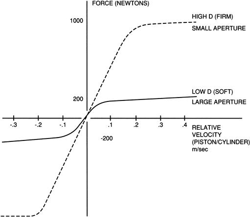
Figure 8.27 Strut force velocity relationship for variable-aperture strut.
Strut damping can also be varied continuously using the hypothetical mechanism above by means of a motor actuator. In this configuration, the force/velocity relationship will be a curve between the solid and dashed curves of Figure 8.27. One control scheme that is potentially approachable to a continuously variable strut damping is based upon monitoring vehicle operational conditions. In this scheme, sensors are provided which continuously monitor vehicle operating conditions. In addition to the lateral acceleration sensor, a solid-state accelerometer is available that can be placed at a convenient location on the car body to measure sprung mass acceleration (as(t)). Calculation of the RMS value ![]() yields an indication of ride. Whenever
yields an indication of ride. Whenever ![]() exceeds a given level (possibly driver adjusted), the control system can generate a signal to operate strut apertures to lower this acceleration. Another accelerometer could be mounted on the unsprung masses (e.g. wheel axle assembly to monitor its acceleration (au(t))). Integration twice with respect to time can give a running measure of displacement:
exceeds a given level (possibly driver adjusted), the control system can generate a signal to operate strut apertures to lower this acceleration. Another accelerometer could be mounted on the unsprung masses (e.g. wheel axle assembly to monitor its acceleration (au(t))). Integration twice with respect to time can give a running measure of displacement:
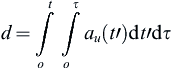 (98)
(98)
Whenever the RMS value of d indicates a potential handling problem, the strut damping could be commanded to optimize handling. Various algorithms are potentially available to set suspension damping to an optimum value with handling probably taking a higher priority over ride in the interest of safety. On the other hand as long as safety is not compromised, ride can be optimized.
Variable Damping via Variable Strut Fluid Viscosity
Variable suspension damping is also achieved with a fixed aperture and variable fluid viscosity. The fluid for such a system consists of a synthetic hydrocarbon with suspended iron particles and is called a magneto-rheological fluid (MR). An electromagnet is positioned such that a magnetic field is created whose strength is proportional to current through the coil. This magnetic field passes through the MR fluid. In the absence of the magnetic field, the iron particles are randomly distributed and the MR fluid has relatively low viscosity corresponding to low damping. As the magnetic field is increased from zero, the iron particles begin to align with the field, and the viscosity increases in proportion to the strength of the field (which is proportional to the current through the electromagnet coil). That is, the damping of the associated shock absorber/strut, which incorporates MR fluid, varies continuously with the electromagnet coil current. Since damping is dependent on both viscosity and the strut aperture, this variable viscosity can be used to optimize damping either alone or in combination with variable aperture. However, in practice, the magnetic fields involved in varying the strut damping over a useful range tend to be large. The entire strut structure must be configured to permit such fields to be generated with practically achievable current levels.
Variable Spring Rate
It was shown above that the frequency response characteristics of a suspension system are influenced by the springs as well as the shock absorber damping. Conventional steel springs (i.e. coil or leaf) have a fixed spring rate (i.e. force–deflection characteristics). For any given set of suspension springs, the vehicle height above the ground is determined by vehicle weight, which in turn depends on loading (i.e. passengers, cargo, and fuel). Some vehicles, having electronically controlled suspension, are also equipped with pneumatic springs as a replacement for steel springs. A pneumatic spring consists of a rubber bladder mounted in an assembly and filled with air under pressure. This mechanism is commonly called an air suspension system.
Unlike metallic springs, however, pneumatic springs have nonlinear force deflection relationship. A pneumatic spring consists of a cylinder/piston assembly with a gas (e.g. nitrogen or air between the end of the piston and the sealed cylinder). A gas under pressure p varies with the volume V of the chamber which contains it in accordance with the adiabatic gas law:
![]() (99)
(99)
where K is the constant and γthe ratio of specific heat at constant pressure to that at constant volume (γ = 1.4 for air).
The pneumatic spring volume V is given by
![]() (100)
(100)
where Ap is the piston cross-sectional area, ![]() is the distance of the piston top surface to the cylinder end at its maximum extension, and x is the displacement due to external force
is the distance of the piston top surface to the cylinder end at its maximum extension, and x is the displacement due to external force ![]() .
.
The force vs. displacement function is given by
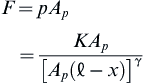 (101)
(101)
As the piston moves toward the end of the cylinder (i.e. increasing x) due to increased normal force on the wheel assembly, the strut force increases nonlinearly with x. This type of gas spring has long been employed in aircraft landing gear structures where the nonlinear force/displacement is beneficial for absorbing vertical loads imparted during landings.
The force vs. displacement rate for such pneumatic springs is proportional to the pressure in the bladder. In automotive suspension springs, a motor-driven pump is normally provided that varies the pressure in the bladder, yielding a variable spring rate suspension. In conjunction with a suitable control system, the pneumatic springs can automatically adjust the vehicle height to accommodate various vehicle loadings, as well as to increase spring “stiffness.”
Electronic Suspension Control System
The control system for an exemplar electronic suspension system is depicted in the block diagram of Figure 8.28.
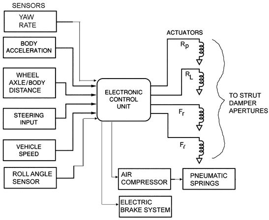
Figure 8.28 Example electronic suspension system configuration.
The control system configuration in Figure 8.28 is generic and not necessarily representative of the system for any production car. This system includes sensors for measuring vehicle speed; steering input (i.e. angular deflection of steered wheels); relative displacement of the wheel assembly and car body/chassis; lateral acceleration; and yaw rate. The outputs are electrical signals to the shock absorber/strut actuators and to the motor/compressor that pressurizes the pneumatic springs (if applicable). The actuators can be solenoid-operated (switched) orifices or motor-driven variable orifices or electromagnets for RH fluid-type variable viscosity struts. Certain vehicles may also be equipped with automatic electrically operated brakes (such as explained in the discussion of ACC) for stability enhancement purposes.
The control system typically is in the form of a microcontroller or microprocessor-based digital controller. The inputs from each sensor are sampled, converted to digital format, and stored in memory. As explained above, the body acceleration measurement can be used to evaluate ride quality. The controller makes this evaluation based upon ![]() or similar metrics for body motion. The relative road/wheel axle displacement d can be used to estimate tire normal force, and damping is then adjusted to try to optimize this normal force.
or similar metrics for body motion. The relative road/wheel axle displacement d can be used to estimate tire normal force, and damping is then adjusted to try to optimize this normal force.
Body roll angle ![]() or the yaw rate sensor (r) provides data which in relationship to vehicle speed and steering input measurements can be used to evaluate cornering performance. In certain vehicles, these measurements combine in an algorithm that is used to activate the electrohydraulic brakes for enhanced stability during extreme maneuvers. The details of automotive stability enhancement is beyond the scope of this book, but the interested reader should refer to Society of Automotive Engineers (SAE) publications on this subject.
or the yaw rate sensor (r) provides data which in relationship to vehicle speed and steering input measurements can be used to evaluate cornering performance. In certain vehicles, these measurements combine in an algorithm that is used to activate the electrohydraulic brakes for enhanced stability during extreme maneuvers. The details of automotive stability enhancement is beyond the scope of this book, but the interested reader should refer to Society of Automotive Engineers (SAE) publications on this subject.
Under program control in accordance with the control strategy, the electronic control system generates output electrical signals to the various actuators. The variable damping actuators vary either the oil passage orifice or the RH fluid viscosity independently at each wheel to obtain the desired damping for that wheel.
There are many possible control strategies and many of these are actually used in production vehicles. For the purposes of this book, it is perhaps most beneficial to present a representative control strategy that typifies features of a number of actual production systems.
The important inputs to the vehicle suspension control system come from road roughness-induced forces and inertial forces (due, for example, to cornering or maneuvering), steering inputs, and vehicle speed. In our hypothetical simplified control strategy, these inputs are considered separately. When driving along a nominally straight road with small steering inputs, the road input is dominant. In this case, the control is based on the spectral content (frequency region) of the relative motion. The controller (under program control) calculates such variables as ![]() or
or ![]() (from the corresponding sensor’s data). Whenever the amplitude of the spectrum near the peak frequencies exceeds a threshold, damping is increased, yielding a firmer ride and improved handling. Otherwise, damping is kept low (soft suspension).
(from the corresponding sensor’s data). Whenever the amplitude of the spectrum near the peak frequencies exceeds a threshold, damping is increased, yielding a firmer ride and improved handling. Otherwise, damping is kept low (soft suspension).
If, in addition, the vehicle is equipped with an accelerometer (usually located in the car body near the center of gravity) and with motor-driven variable-aperture shock absorbers, then an additional control strategy is possible. In this latter control strategy, the shock absorber apertures are adjusted to minimize sprung mass acceleration in the 2–8 Hz frequency region, thereby providing optimum ride control. However, at all times, the damping is adjusted to control unsprung mass motion to maintain wheel normal force variation at acceptably low levels for safety reasons. Whenever a relatively large steering input is sensed (sometimes in conjunction with body roll angle and/or yaw rate measurement), such as during a cornering maneuver, then the control strategy switches to the smaller aperture, yielding a “stiffer” suspension and improved handling. In particular, the combination of cornering on a relatively rough road calls for damping that optimizes tire normal force, thereby maximizing cornering forces.
Electronic Steering Control
The steering system of a car consists of a mechanism for rotating the front wheels of the car about an axis that is nearly vertical in response to steering wheel angle changes. The basic mechanism is shown schematically in Figure 8.29.
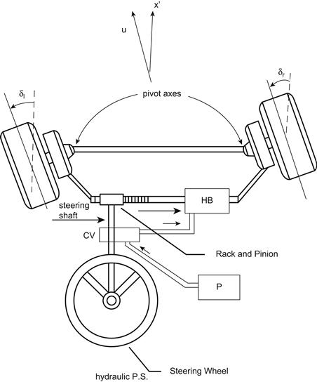
Figure 8.29 Basic steering mechanism with power assist.
The force/torque of the steering wheel is influenced by the actual orientation of the pivot axes relative to the car body vertical axis. The fore/aft angle is known as camber angle. An increase in this angle relative to vertical increases steering torque; it also increases restoring torque, which tends to rotate the wheels toward the body symmetry plane after a turn has been completed. Typically, the camber angle is only a few degrees, but this angle in combination with the lateral orientation of the pivot axis (known as caster angle) is beneficial in steering stability. Proper alignment of these angles assists the vehicle in tracking a straight heading for neutral steering torque.
The adverse effect of this wheel alignment is an increase in steering effort for the driver relative to zero camber and caster, which is undesirable. Rather than compromise on alignment to achieve lower steering effort, car manufacturers have found it desirable to provide a power assist via a hydraulic system as depicted in Figure 8.29. An engine-driven pump P provides hydraulic fluid (power steering fluid) under pressure. This pressurized fluid is sent via hydraulic lines to a control valve (CV) mounted at some point on the steering shaft. This CV directs the pressurized fluid to a hydraulic cylinder mechanism that applies torque in the same direction as the steering wheel.
A basic problem with such a system comes from matching the desired boost with that available from the power steering pump. Figure 8.30 shows qualitatively the desired boost which decreases with vehicle speed.
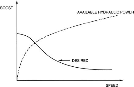
Figure 8.30 Power steering boost vs. speed.
Unfortunately in early power steering systems, the available boost was an increasing function of engine speed (owing to the increase in pump speed with engine speed) which is a function of vehicle speed and the transmission gear ratio. Although it is possible to obtain a constant boost with respect to engine RPM via pressure regulating valves yielding a constant boost with respect to vehicle speed, obtaining desired boost was not readily achievable with purely mechanical systems. On the other hand, electronic controls provide a relatively straightforward means of regulating boost to obtain desired results. Moreover, a digital power steering control system allows for the possibility of changing the boost vs. speed profile via software changes. A control that adapts automatically to driving conditions is also achievable cost effectively. In an electrohydraulic power steering system the hydraulic pressure to the boost cylinder can be varied via an adjustable pressure relief valve. An actuator for such a system can be a motor (e.g. stepper motor) or a solenoid, possibly driven by a variable-duty-cycle control signal (see Chapter 6).
An alternative power steering scheme uses a special electric motor to provide the boost required instead of the hydraulic boost as depicted in Figure 8.31.
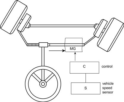
Figure 8.31 Electric power steering boost.
In this figure, a motor gear system is coupled to the steering mechanism in such a way as to provide the torque boost. A digital control system C receives vehicle speed measurements via speed sensors and generates a motor control signal to achieve the desired speed/boost profile. Electric boost power steering has several advantages over traditional hydraulic power steering. Electronic control of electric boost systems is straightforward and can be accomplished without any energy conversion from electrical power to mechanical actuation. Moreover, electronic control offers very sophisticated adaptive control in which the system can adapt to the driving environment. A basic problem with a direct electric motor steering boost is that an electric motor must be rotating to produce meaningful torque. For any driving situation in which a constant steering angle input is required (e.g. for vehicle moving along an arc of constant radius of curvature), the motor would have to generate the torque boost while not rotating. An alternative electric boost scheme involves an electric motor directly driving a hydraulic pump that is part of an electrohydraulic power steering system.
Four-Wheel Steering
Electronically controlled power steering also has the capability for four-wheel steering (4WS). As will be shown later 4WS be highly useful during vehicle curb parking but also has potential for improved road maneuverability. An example of an electronically controlled steering system that has had commercial production is for four-wheel steering systems (4WS). In the 4WS-equipped vehicles, the front wheels are directly linked mechanically to the steering wheel, as in traditional vehicles. There is a power steering boost for the front wheels as in a standard two-wheel steering system. The rear wheels are steered under the control of a microcontroller via an actuator. Figure 8.32 is an illustration of the 4WS configuration.
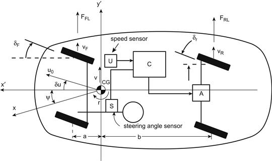
Figure 8.32 4WS basic configuration.
In Figure 8.32, the notation is as follows:
x′ = vehicle longitudinal axis
x = inertial (ECEF) reference axis (i.e. initial direction of ![]() )
)
δF = angle between ![]() and the front tire plane of symmetry
and the front tire plane of symmetry
δR = angle between ![]() and the rear tire plane of symmetry
and the rear tire plane of symmetry
uo = car instantaneous velocity vector
a = longitudinal distance CG to front wheel axis
b = longitudinal distance CG to rear wheel axis
vF = lateral velocity of front wheel relative to road surface
vR = lateral velocity of rear wheel relative to road surface
During ordinary driving of a passenger car the angle between the car longitudinal axis and the instantaneous velocity vector (δu) is small such that ![]() ,
, ![]() . Under these conditions, the lateral velocities of the front and rear tires respectively are given by
. Under these conditions, the lateral velocities of the front and rear tires respectively are given by
![]() (102)
(102)
The models for the tire lateral forces at the front and rear tires FFL and FRL respectively are based on the so-called tire slip angles αF and αR respectively. Neglecting the small angle δu, these are the angles between the vehicle longitudinal axis ![]() and the instantaneous velocity vector of the tire contact point with the road and are given by
and the instantaneous velocity vector of the tire contact point with the road and are given by
 (103)
(103)
In these equations right-and-left symmetry is assumed which is valid for relatively small δF, δR such as is the case while driving on the highway. It is consistent with the small-angle assumptions that these angles are given approximately by
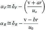 (104)
(104)
For a conventional front wheel steering car, δR = 0. The tire lateral or so-called cornering forces (for small angles) FFL (front) and FRL (rear) and front wheel steering are given by
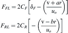 (105)
(105)
where CF is the front tire concerning stiffness, CR the rear tire concerning stiffness, and where right/left symmetry is assumed.
The cornering stiffness is a steering parameter, which is a function of the tire characteristics and road surface. It is also a function of the instantaneous tire normal force (i.e. NF, NR). However, for the present discussion, it is assumed to be a constant for the following steering maneuver.
The model for lateral translational motion is found by summing forces acting in the y′-direction:
![]() (106)
(106)
where M is the vehicle mass.
Similarly, the model for the rotational motion about the CG is found by summing all moments about the CG and is given by
![]() (107)
(107)
where Izz is the vehicle moment of inertia about the vertical axis through the CG.
The motion of the car in response to a steering input δF(t) is found by solving the above equations. The solution for any set of coupled linear first-order equations is facilitated using state variable approach as explained in Chapter 1. In this case the independent variables v,r are put in state vector (x) form where the state vector is given by
![]() (108)
(108)
The state variable model for the pair of equations is in the form
![]() (109)
(109)
where the state transition matrix A is given by
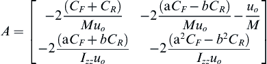
and the input matrix B is given by
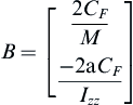 (110)
(110)
The input u for front wheel steering is given by
![]() (111)
(111)
Taking the Laplace transform of the state variable Eqn (109) and solving for x(s) yields
![]() (112)
(112)
where I is an identity matrix which, for a two-dimensional vector, is given by
![]()
Solution of the equation for x(s) is straightforward once the parameters of the A and B matrix are determined for any given vehicle, set of tires and steering command. As shown in Chapter 1 the time domain state vector can be readily found using inverse Laplace (i.e. residue) methods.
The simplified steering model above for front wheel steering has ignored vehicle roll dynamics during a steering maneuver. We next develop a model for a 4WS (with electronic controls and for which δR can be nonzero) that includes roll dynamics. In writing a set of equations that includes roll, it is necessary to distinguish sprung mass (Ms) from unsprung mass (Mu) and total vehicle mass (M) where
![]()
Summing the forces acting in the y′-direction through the CG yields the following equation:
![]() (113)
(113)
where the possibility of nonzero δR is explicitly taken. Summing moments about the vertical axis through the CG yields the following equation:
![]() (114)
(114)
where the cross-moment of inertia Izx has not been neglected. Finally, summing moments about the longitudinal axis through the CG yields the following equation:
![]() (115)
(115)
where
and
The above set of coupled linear differential equations can be written in state variable form with a four-dimensional state vector
 (116)
(116)
and input vector
![]()
This equation is four dimensional requiring four coupled differential equations. In addition to the three given above, the 4th differential equation is given by
![]()
The state vector equation is given by
![]() (117)
(117)
The matrix G is given by
 (118)
(118)
The matrix H is given by

and matrix D is given by

The above state variable equation can be put in standard form by multiplying Eqn (117) by the inverse of G yielding
![]()
where
In the illustration of Figure 8.32, the front wheels are steered to a steering angle δF by the driver’s steering wheel input. A sensor (S) measures the steering angle and another sensor (U) gives the vehicle speed. The microcontroller (C) determines the desired rear steering angle δR under program control as a function of speed and front steering angle via actuator A.
In an exemplary 4WS control strategy for speeds below 10 mph, the rear steering angle is in the opposite direction to the front steering angle. This control strategy has the effect of decreasing the car’s turning radius by as much as 30% from the value it has for front wheel steering only. Consequently, the maneuvering ability of the car at low speeds is enhanced (e.g. for parking).
At intermediate speeds (e.g. 11 mph < U < 30 mph), the steering might be front wheel only. At higher speeds (including highway cruise), the front and rear wheels are steered in the same direction. At least one automaker has an interesting strategy for higher speeds (e.g. at highway cruise speed). In this strategy, the rear wheels turn in the opposite direction to the front wheels for a very short period (on the order of 1 s) and then turn in the same direction as the front wheels. This strategy has a beneficial effect on maneuvers such as lane changes on the highway.
As an illustration of the influence of electronic 4WS on vehicle maneuvers, a simulation has been run on a hypothetical vehicle having the following metric system parameters:
Figure 8.33 qualitatively depicts the car position during alone change maneuver for 2Ws and for 4Ws.

Figure 8.33 Lane change maneuver (qualitative sketch).
From the simulation, Figure 8.34 plots the steering wheel angle in radians for this lane change-type maneuver as well as the vehicle lateral motion y(t) of the CG. The control strategy in this simulation is for the rear wheel deflection ![]() . The solid curve represents 4WS response and the dashed curve the response for 2WS. Note that the lane change amount is twice as much for 4WS as for 2WS during the steering input time interval. Alternatively a given lateral displacement can be achieved in half the time with 4WS as for 2Ws.
. The solid curve represents 4WS response and the dashed curve the response for 2WS. Note that the lane change amount is twice as much for 4WS as for 2WS during the steering input time interval. Alternatively a given lateral displacement can be achieved in half the time with 4WS as for 2Ws.

Figure 8.34 Lane change maneuver 4WS vs. 2WS from simulation.
This simulation of a lane change maneuver with rear wheels steered in the opposite direction is only intended to illustrate the significant differences in maneuvering for 4WS compared to 2WS. In fact, such a control strategy is not necessarily desirable for passenger car electronically controlled 4WS. Rather it might be more appropriate for certain race car applications.
For normal passenger cars, it is more likely that at highway cruise speeds the rear wheel steering would be in the same direction as the front wheels but at a somewhat smaller peak deflection. Another passenger car control strategy might be to steer the rear wheels opposite to the front wheels for a short period and then to steer them in the same direction (although at a smaller angle). Many control strategies can be evaluated in simulation using models such as are presented above or (preferably) more accurate models than above with respect to nonlinearities and un-modeled dynamics.
Turning the wheels in the same direction at cruising speeds has another benefit for a vehicle towing a trailer. When front and rear wheels turn in the same direction, the angle between the car and trailer axes is less than it is for front wheel steering only. The reduction in this angle means that the lateral force applied to the rear wheels by the trailer in curves is less than that for front wheel only steering. This lateral force reduction improves the stability of the car or truck/trailer combination relative to front steering only.
Summary
This chapter has reviewed some basic theory for vehicle-motion control. In practice and in production vehicles, the models presented here would not be adequate for development of actual control systems. However, the relevant models involve very complicated nonlinear, coupled differential equations that extend beyond the intended scope of this book. On the other hand, the simplified models presented here illustrate the theory of such complex electronic systems. There is abundant literature available through the Society of Automotive Engineers (SAE) and its publication services for the reader who is interested in pursuing the advanced theory of vehicle-motion control. It is hoped that the discussions in this chapter have prepared the reader well enough to be able to understand these publications.