Chapter 7
Digital Powertrain Control Systems
Chapter Outline
Digital Engine Control Features
Control Modes for Fuel Control
Discrete Time Idle Speed Control
Spark Advance Correction Scheme
Integrated Engine Control System
Evaporative Emissions Canister Purge
Automatic Transmission Control
Torque Converter Lock-Up Control
Differential and Traction Control
Introduction
Traditionally, the term powertrain has been used to include the engine, transmission, differential, and drive axle/wheel assemblies. With the advent of electronic controls, the powertrain also includes the electronic control system (in whatever configuration it has). In addition to engine control functions for emissions regulation, fuel economy, and performance, electronic controls are also used in the automatic transmission to select shifting as a function of operating conditions. Moreover, certain vehicles employ electronically controlled clutches in the differential (transaxle) for traction control. Electronic controls for these major powertrain components can be either separate (i.e., one for each component) or an integrated system regulating the powertrain as a unit.
This latter integrated control system has the benefit of obtaining optimal vehicle performance within the constraints of exhaust emission and fuel economy regulations. Each of the control systems is discussed separately beginning with electronic engine control. Then a brief discussion of integrated powertrain follows. This chapter concludes with a discussion of hybrid, electric vehicle (HEV) control systems in which propulsive power comes from an IC engine or an electric motor, or a combination of both. The proper balance of power between these two sources is a complex function of operating conditions and governmental regulations.
Digital Engine Control
Chapter 5 discussed some of the fundamental issues involved in electronic engine control. This chapter explores some practical digital control systems. There is, of course, considerable variation in the configuration and control concept from one manufacturer to another. However, this chapter describes representative control systems that are not necessarily based on the system of any given manufacturer, thereby giving the reader an understanding of the configuration and operating principles of a generic representative system. As such, the systems in this discussion are a compilation of the features used by several manufacturers.
In Chapter 5, engine control was discussed with respect to continuous time representation. In fact, modern engine control systems, such as the ones discussed in this chapter, are digital. A typical engine control system incorporates a microprocessor and is essentially a special-purpose computer (or microcontroller).
Electronic engine control has evolved from a relatively rudimentary fuel control system employing discrete analog components to the highly precise fuel and ignition control achieved through microprocessor-based integrated digital electronic powertrain control. The motivation for development of the more sophisticated digital control systems has been the increasingly stringent exhaust emission and fuel economy regulations that have evolved recently. It has proven to be cost effective to implement the powertrain controller as a multimode computer-based system to satisfy these requirements.
A multimode controller operates in one of many possible modes, and, among other tasks, changes the various calibration parameters as operating conditions change in order to optimize performance. To implement multimode control in analog electronics, it would be necessary to change hardware parameters (for example, via switching systems) to accommodate various operating conditions. In a computer-based controller, however, the control law and system parameters are changed via program (i.e., software) control. The hardware remains fixed but the software is reconfigured in accordance with operating conditions as determined by sensor measurements and switch inputs to the controller.
This chapter will explain how the microcontroller under program control is responsible for generating the electrical signals that operate the fuel injectors and trigger the ignition pulses. This chapter also discusses secondary functions (including management of secondary air that must be provided to the catalytic converter, EGR regulation, and evaporative emission control) that have not been discussed in detail before.
All digital systems are inherently discrete time model based. That is, rather than modeling systems or subsystems on a continuous time basis, all processes are characterized at discrete times tk where
![]() (1)
(1)
The time interval between successive sample times is the period during which the control system performs the necessary computations to perform its function. The theoretical basis for discrete time system modeling and analysis has been explained in Chapter 2. However, as explained in Chapter 5, the majority of automotive control or instrumentation systems employ some analog sensors and actuators (or in the instrumentation case, displays).
In Chapter 6, it was shown that the majority of sensors and actuators are analog devices that are modeled as functions of continuous time t. As described in Chapter 2, measurements made by continuous time sensors are sampled at times tk to obtain the necessary discrete time system input. When representing the sampled data from a continuous time sensor having an output terminal voltage V0(t) the notation used here to represent the kth sample of V0 is Vk where
![]() (2)
(2)
It is, perhaps, worthwhile at this point to illustrate the operation of a digital control system with a simple example. Although certain automotive control requires measurements from multiple sensors (i.e. with multiple inputs) to perform a specific task, our illustration considers the example of a single input, single output (SISO) linear system. Let the input to the controller at time tk be xk and the output corresponding to this and other previous inputs be denoted yk. It should be noted that yk is output from the digital system at a time delayed from the xk owing to the nonzero computation time. As explained in Chapter 2, one form for the relationship between the input and output of a linear SISO digital system is given by the recursive algorithm below:
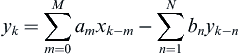 (3)
(3)
The coefficients am and bn are chosen by the designer to perform a specific task. It should be noted that for a purely linear system with continuous time sensor and actuator, it is possible to develop the control function relating input and output using continuous time techniques. Then the discrete time coefficients can be obtained from this continuous time function by a discretization process as described in Chapter 2.
The trend in contemporary automotive electronic systems is to perform multiple control operations using an integrated digital system based upon a microprocessor/microcontroller. Furthermore, it is an aspect of a digital system that nonlinear transformations and/or calculations are handled as well as linear ones.
Digital Engine Control Features
Recall from Chapter 5 that one primary purpose of the electronic engine control system is to regulate the mixture (i.e., air–fuel), the ignition timing, and EGR. Virtually all major manufacturers of cars sold in the United States (both foreign and domestic) use the three-way catalytic converter for meeting exhaust emission constraints. For such cars, the air/fuel ratio is held as closely as possible to the stoichiometric value of about 14.7 for as much of the time as possible. Ignition timing and EGR are controlled separately to optimize performance and fuel economy.
Figure 7.1 illustrates the primary components of an electronic engine control system. In this figure, the engine control system is a microcontroller, typically implemented with a specially designed microprocessor or microcontroller and operating under program control. Spark plugs for this four-cylinder example are denoted S.P.
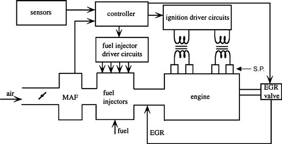
Figure 7.1 Components of an electronically controlled engine.
Typically, the controller incorporates hardware for the multiply/divide operation as well as ROM (see Chapter 4). The hardware multiply greatly speeds up the multiplication routines, which are generally cumbersome and slow when implemented by a subroutine in the software. The associated ROM contains the program for each mode as well as calibration parameters and lookup tables. The microcontroller under program control generates output electrical signals to operate the fuel injectors so as to maintain the desired mixture and ignition to optimize performance. For a given engine output power (as commanded by the driver via the accelerator pedal), the correct mixture is obtained by regulating the quantity of fuel delivered into each cylinder during the intake stroke in accordance with the corresponding intake air mass, as explained in Chapter 5.
With respect to the fuel control function the digital engine control system obtains a measurement of mass airflow typically using a mass airflow (MAF) sensor. As shown in Chapter 6, the MAF sensor generates an output terminal voltage vo given by
![]() (4)
(4)
where ![]() is the instantaneous mass airflow rate into the engine intake system (kg/s).
is the instantaneous mass airflow rate into the engine intake system (kg/s).
As explained in Chapter 6, the function Fm for a representative production MAF sensor is given by
![]()
However, a digital fuel control system can invert a nonlinear function to obtain the value ![]() of mass airflow:
of mass airflow:
![]() (5)
(5)
As explained in Chapter 5, the intake to the engine includes EGR as well as air. As will be shown below, the digital engine control system is able to determine the EGR mass flow rate ![]() since it controls the flow of EGR. In certain cases, the EGR rate is determined from a differential pressure sensor (DPS). Thus, the correction for
since it controls the flow of EGR. In certain cases, the EGR rate is determined from a differential pressure sensor (DPS). Thus, the correction for ![]() in the MAF sensor output is a straightforward computation.
in the MAF sensor output is a straightforward computation.
An ideal engine control would determine the mass of air drawn into the mth cylinder during the nth engine cycle Ma(n, m). This ideal controller would instantaneously inject fuel with a uniform distribution at the end of the intake process for this cylinder to achieve a uniform stoichiometric mixture throughout the cylinder in preparation for compression ignition and power generation. This ideal process would assure that all cylinders achieved the desired stoichiometric mixture for each cycle as desired for optimum exhaust emissions in conjunction with the catalytic converter. However, this ideal fuel control is not practically achievable.
On the other hand, suboptimal fuel control that is very close to optimal can be achieved in practice. As will be shown later in this chapter, closed-loop fuel control provides sufficient regulation of mixture to meet the strictest emission regulations. It will also be shown later in this chapter that fuel control operates in several possible modes. However, before proceeding to this discussion it is helpful to explain some of the basic issues in the development of the final system configuration and fuel control algorithms.
In practice, an MAF sensor is placed somewhere in the upstream end of the engine intake system of tubes that direct airflow to the individual cylinders. Typically, this intake system (called “the intake manifold”) is designed to achieve as uniform as possible a distribution among all cylinders over the broadest possible operating range. For the present discussion, it is helpful to assume that a uniform distribution of air is achieved for each engine cycle.
At any instant t the total mass of air pumped into the engine during the previous engine cycle of duration Te (corresponding to crankshaft rotation through 4π rotations) is given by
 (6)
(6)
where θe(t) is the crankshaft instantaneous angular position at time t and Te is the period of an engine cycle at the instantaneous RPM
![]()
For simplification and without serious loss of generality it is convenient to assume that the engine is operating at a steady load and RPM. According to our assumptions, the amount of air drawn into any given cylinder (m) during the nth engine cycle Ma(n, m) is given by
![]() (7)
(7)
where Mc is the number of cylinders.
Note: If the RPM and load are changing but at a slow enough rate, then for at least the period of one cycle the above model is sufficiently accurate to compute the desired fuel delivery for a stoichiometric mixture.
The fuel mass to be supplied to cylinder m during the nth engine cycle f(n,m) is given by
![]() (8)
(8)
where Ra/f is the desired ratio of mass of air to mass of fuel. As explained below, the correct Ra/f depends upon the control operating mode. It is desirable that Ra/f be at stoichiometry (i.e., Ra/f = 14.7) for as much of the engine-operating period as possible for optimum exhaust emission regulation.
As explained in Chapter 6, fuel delivery in contemporary engines is provided by fuel injectors. It should be recalled that a fuel injector is a solenoid-operated valve that is opened by an electrical control signal at the proper time in the engine cycle for a period of time τf(n, m) (for cylinder m during cycle n) that is computed in the digital engine control system. It was also explained in Chapter 6 that fuel under a regulated pressure is available on the upstream side of the fuel injector valve via the fuel rail.
The fuel flow rate ![]() is a function of the fuel rail pressure as well as the open area of the valve and the displacement of the pintle by the solenoid. These latter two parameters are fixed by the structure of the fuel injector. The quantity of fuel delivered by the fuel injector F(n, m) for the mth cylinder during the nth engine cycle is given by
is a function of the fuel rail pressure as well as the open area of the valve and the displacement of the pintle by the solenoid. These latter two parameters are fixed by the structure of the fuel injector. The quantity of fuel delivered by the fuel injector F(n, m) for the mth cylinder during the nth engine cycle is given by
 (9)
(9)
where tn,m is the beginning time of fuel delivery control binary signal, tn,m + τF(n, m) is the end of fuel injection period, and ![]() is the fuel flow rate for fuel injector.
is the fuel flow rate for fuel injector.
It is common practice in contemporary engine design to place the fuel injector near to the intake valve such that the fuel spray during the fuel injector open period is directed into the cylinder through the intake valve opening. The binary fuel injection control voltage is timed such that fuel is delivered during a portion of the intake stroke.
The fuel injector opening and closing dynamics are sufficiently short except for very small F(n, m) that the fuel delivery is given approximately by
![]() (10)
(10)
It should be noted that for steady load and RPM typically τF should be constant; however, for varying load and accelerating/decelerating engine τF may vary with both n and m. Consequently, the notation τF retains both indices.
Control Modes for Fuel Control
The engine control system is responsible for controlling fuel and ignition for all possible engine-operating conditions. However, there are a number of distinct categories of engine operation, each of which corresponds to a separate and distinct operating mode for the engine control system. The differences between these operating modes are sufficiently great that a different software routine may be used for each. The control system must determine the operating mode from the existing sensor data and call the particular corresponding software routine. We begin with a qualitative survey of system operation in the various control modes and later present formal models.
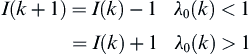
For a typical engine, there are at least seven different engine-operating modes that affect fuel control: engine crank, engine warm-up, open-loop control, closed-loop control, hard acceleration, deceleration, and idle. The program for mode control logic determines the engine-operating mode from sensor data and timers.
In the earliest versions of electronic fuel control systems, the fuel metering actuator typically consisted of one or two fuel injectors mounted near the throttle plate so as to deliver fuel into the throttle body. These throttle body fuel injectors (TBFIs) were in effect an electromechanical replacement for the carburetor. Requirements for the TBFI were such that they only had to deliver fuel at the correct average flow rate for any given mass airflow rate. Mixing of the fuel and air, as well as distribution to the individual cylinders, took place in the intake manifold system.
The more stringent exhaust emissions regulations of recent years have demanded more precise fuel delivery than can normally be achieved by TBFI. These regulations and the need for improved performance have led to timed sequential port fuel injection (TSPFI). In such a system, there is a fuel injector for each cylinder that is mounted so as to spray fuel directly into the intake of the associated cylinder.
For the purposes of the present discussion, fuel delivery is assumed to be TSPFI (i.e., via individual fuel injectors located so as to spray fuel directly into the intake port and timed to coincide with the intake stroke). Airflow measurement is via an MAF sensor. Some engine control systems involve vehicle speed sensors and various switches to identify brake on/off and the transmission gear, depending on the particular control strategy employed. We consider next the individual engine control modes.
Engine Start
When the ignition key is switched on initially, the mode control logic automatically selects an engine start control scheme that provides the correct temperature-dependent air/fuel ratio required for starting the engine. Once the engine RPM rises above the cranking value, the controller identifies the “engine started” mode and passes control to the program for the engine warm-up mode. This operating mode typically keeps the air/fuel ratio relatively low to prevent engine stall during cool or cold weather until the engine coolant temperature rises above some minimum value. The instantaneous desired air/fuel is a function of coolant temperature and ambient conditions. The particular value for the minimum coolant temperature is specific to any given engine type and, in particular, to the fuel metering system. (Alternatively, the low air/fuel ratio may be maintained for a fixed time interval following start, depending on start-up engine temperature.)
Open-Loop Mode
When the coolant temperature rises sufficiently, the mode control logic directs the system to operate in the open-loop control mode until the EGO sensor warms up enough to provide accurate readings. This condition is detected by monitoring the EGO sensor’s output for voltage readings above a certain minimum rich air/fuel mixture voltage set point (see Chapter 6 for EGO sensor voltage characteristics). When the sensor has indicated rich at least once and after the engine has been in open loop for a specific time, the control mode selection logic selects the closed-loop mode for the system. (Note: other criteria may also be used.) The engine remains in the closed-loop mode until the EGO sensor cools and fails to read a rich mixture for a certain length of time or a hard acceleration or deceleration occurs. If the sensor cools, the control mode logic selects the open-loop mode again.
Acceleration/Deceleration
During hard acceleration or heavy engine load, the control mode selection logic chooses a scheme that provides a rich air/fuel mixture for the duration of the acceleration or heavy load. This scheme has the capability to provide maximum torque, but depending on driver demand, suboptimal emissions control, and relatively poor fuel economy regulation as compared with a stoichiometric air/fuel ratio may occur. After the need for enrichment has passed, control is returned to either open-loop or closed-loop mode, depending on the control mode logic conditions that exist at that time. During periods of deceleration, the air/fuel ratio might be increased to reduce emissions of HC and CO due to unburned excess fuel. However, enleanment is limited to an air/fuel that avoids excess NOx production.
When idle conditions are present, control mode logic passes system control to the idle speed control mode. In this mode, the engine speed is controlled to reduce engine roughness and stalling that might occur because the idle load has changed due to air conditioner compressor operation, alternator operation, or gearshift positioning from park/neutral to drive, although stoichiometric mixture is used if the engine is warm. A detailed model and performance analysis of idle speed control is presented later in this chapter.
As explained above, in modern engine control systems, the controller is a special-purpose digital computer built around a microprocessor or microcontroller. An exemplary configuration of a typical modern digital engine control system is depicted in Figure 7.2.

Figure 7.2 Digital engine control system diagram.
The controller also includes ROM containing the main program (of several thousand lines of code). This ROM is accessed by the engine control system via address bus A and receives data via data bus D (see Chapter 4). There is also a section of ROM continuing parameter values for specific control modes and tables of data for various control functions as explained later in this chapter. Of course, any microprocessor-based system must have RAM for temporary storage of data during computation (see Chapter 4). The sensor signals are connected to the controller via an input/output (I/O) subsystem. Similarly, the I/O subsystem provides the output signals to drive the fuel injectors (shown as the fuel metering block of Figure 7.2) as well as to trigger pulses to the ignition system (described later in this chapter). In addition, this microprocessor-based control system includes hardware for sampling and analog-to-digital conversion such that all sensor measurements are in a format suitable for reading by the microprocessor. (Note: See Chapter 4 for a detailed discussion of these components.)
With reference to Figure 7.2, the sensors that measure various engine variables for control are as follows:
engine temperature as represented by coolant temperature (CT),
one or two heated exhaust gas oxygen sensor(s) (HEGO),
crankshaft angular position and RPM sensor (CPS),
camshaft position sensor for determining start of each engine cycle (CS POS/RPM),
throttle position sensor (TPS), and
differential pressure sensor (exhaust to intake) for EGR control (DPS).
Other sensors that might be used on older model cars that are not given in Figure 7.2 include the following:
The control system selects an operating mode based on the instantaneous operating condition as determined from the sensor measurements. Within any given operating mode, the desired air/fuel ratio (A/F)d is selected. The controller then determines the quantity of fuel to be injected into each cylinder during each engine cycle. This quantity of fuel depends on the particular engine-operating condition as well as the controller mode of operation, as will presently be explained.
Engine Crank
While the engine is being cranked, the fuel control system must provide an intake air/fuel ratio of anywhere from 2:1 to 12:1, depending on engine temperature. The lowest value for [A/f]d would be applied for very cold temperatures. The correct air/fuel ratio (i.e., [A/F]d) is selected from an ROM lookup table with interpolation (as explained later in this chapter) as a function of coolant temperature. Low temperatures affect the ability of the fuel metering system to atomize or mix the incoming air and fuel properly to achieve combustion. At low temperatures, the fuel tends to form into large droplets in the air, which do not burn as efficiently as tiny droplets. The larger fuel droplets tend to increase the apparent air/fuel ratio, because the amount of usable fuel (on the surface of the droplets) in the air is reduced; therefore, the fuel metering system must provide a decreased air/fuel ratio to provide the engine with a more combustible air/fuel mixture. During engine crank the primary issue is to achieve engine start as rapidly as possible. Once the engine is started the controller switches to an engine warm-up mode.
Engine Warm-Up
While the engine is warming up, an enriched air/fuel ratio relative to stoichiometry is still needed to keep it running smoothly, but the required air/fuel ratio changes as the temperature increases. Therefore, the fuel control system stays in the open-loop mode, but the air/fuel ratio commands continue to be altered due to the temperature changes. The emphasis in this control mode is on rapid and smooth engine warm-up. Fuel economy and emission control may be still a secondary concern. The controller selects a warm-up time from a lookup table based on the temperature of the coolant. In certain cases, a fully warmed engine is switched off by the driver for a brief period such that temperature remains sufficiently high that warm-up mode is either very short or not used at all.
A diagram illustrating the lookup table selection of desired air/fuel ratios is shown in Figure 7.3. Essentially, the measured coolant temperature (Tc) is converted to an address for the lookup table with interpolation as described below. This address is supplied to the ROM table via the system address bus (A/B). The data stored at this address in the ROM are desired air/fuel ratio (A/F)d for the temperature. These data are sent to the controller via the system data bus (D/B).

Figure 7.3 Illustration of table lookup.
The term lookup table refers to obtaining an output variable y that is a function of one or more inputs. It provides an alternative to calculation based upon a model (e.g., a polynomial model). It is often applied to empirically obtained data (e.g., from engine mapping) in which the optimum value of a variable (e.g., air/fuel) has been determined from measurements for various values of the independent variables. It is inherently limited to a finite number of discrete points in the relevant range for the independent variables.
On the other hand, during actual engine operation these same independent variables are continuous and rarely coincide perfectly with the stored values. In this case, the output variable corresponding to these independent variables is obtained by a process called interpolation. This process involves fitting the region between two successive data points with a function (normally linear). We illustrate linear interpolation with a two-dimensional data set. Let yn be the value of a dependent variable (e.g. air/fuel) at independent data sensor output point xn where n = 1,2…N. Let x be a measurement of independent variable (e.g., coolant temperature) for which the corresponding dependent variable y (e.g., desired air/fuel) is sought. Also, let xm and xm+1 be the nearest tabulated data points in the table in which xm < x < xm+1. The corresponding tabulated values for the dependent variable are ym and ym+1. For linear interpolation it is assumed that y varies linearly with x over the domain ![]() . The slope S over this domain is given by
. The slope S over this domain is given by
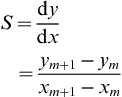 (11)
(11)
The linearly interpolated value for y is given by
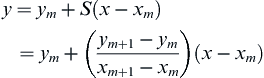 (12)
(12)
Alternatively, it is possible to obtain a polynomial model which gives the best fit to measured data in a least squared error sense. Let an empirical data set be given by {xn, yn: n = 1,2…N}. The polynomial which best represents this data is of the form
![]() (13)
(13)
The mean squared error between this polynomial and the data is
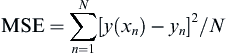 (14)
(14)
There are many computer programs for finding the coefficient set {am: m = 0,1…M} such that MSE is minimized. For example, the MATLAB function polyfit (xn, yn, M) returns the coefficient set am (of order M), which yields the least MSE for the given data set. In this case, the digital engine control can calculate the desired dependent variable for any given measurement of the independent variable x. The choice between table lookup with interpolation and polynomial calculation can be assessed by the quality of fit of the polynomial to the data given by the MSE for the best polynomial fit and by the relative complexity of the two methods. The set of coefficients for any given data are normally determined during the development of an engine control system. These coefficients are stored in ROM such that the determination of y for any measurement x (during normal engine operation) is readily implemented in the control system using Eqn (13) and the stored values for {am} for the polynomial model method and by Eqn (12) for the lookup table and interpolation method.
Returning to the discussion of coolant temperature for setting (A/F)d, there is always the possibility of a coolant temperature failure. Such a failure could result in excessively rich or lean mixtures, which can seriously degrade the performance of both the engine and the three-way catalytic converter (3 wcc). One scheme that can circumvent a temperature sensor failure involves having a time function to limit the duration of the engine warm-up mode. The nominal time to warm the engine from cold soak at various temperatures is known. The controller is configured to switch from engine warm-up mode to an open-loop (warmed-up engine) mode after a sufficient time by means of an internal timer.
Open-Loop Control
For a warmed-up engine, the controller will operate in an open loop if the closed-loop mode is not available for any reason. For example, the engine may be warmed sufficiently but the EGO sensor may not provide a usable signal. In any event, as soon as possible it is important to have a stoichiometric mixture to minimize exhaust emissions.
It was shown above that the quantity of fuel to be delivered to cylinder m during the nth engine cycle can be computed from MAF sensor measurements and can be regulated by means of a fuel injector pulse duration τF(n, m). For the present, it is helpful to assume that intake air is uniformly distributed to all M cylinders. In this case, the fuel injector open duration is
![]() (15)
(15)
This quantity of fuel is actually delivered to each cylinder during the open-loop mode and is often termed the “base pulse duration.” Until conditions permit closed-loop mode of fuel control the fuel quantity is determined from MAF measurements. As a means of denoting open-loop operation the notation for base pulse duration is τb(n):
![]() (16)
(16)
Corrections of the base pulse width occur whenever any conditions affect the accuracy of the fuel delivery. For example, low battery voltage might affect the pressure in the fuel rail that delivers fuel to the fuel injectors. Corrections to the base pulse width are then made using the actual battery voltage.
Closed-Loop Control
Perhaps the most important adjustment to the fuel injector pulse duration comes when the control is in the closed-loop mode. In the open-loop mode, the accuracy of the fuel delivery is dependent upon the accuracy of the measurements of the important variables (e.g., MAF). However, any component of a given physical system is susceptible to changes with operating conditions (e.g., temperature) or with time (aging or wear of components). Such failures or degradation of sensor/actuator calibration can adversely affect exhaust emissions in the open-loop mode.
To avoid degraded emission control, it is important for the control system to switch to the closed-loop mode as soon as possible and to remain in this mode for as much of the engine operation as possible. The closed-loop mode can only be activated when the EGO (or HEGO) sensor is sufficiently warmed. Recall from Chapter 6 that for a fully warmed EGO sensor, the output voltage of the sensor is high (approximately 1 V) when the exhaust oxygen concentration is low (i.e., for a rich mixture relative to stoichiometry). The EGO sensor voltage is low (approximately 0.1 V) whenever the exhaust oxygen concentration is high (i.e., for a mixture that is lean relative to stoichiometry).
Chapter 1 presented a discussion of the theory of the closed-loop control of a dynamic system in which a measurement of the dynamic system output variable that is being regulated/controlled is compared with the desired value. The controller produces an input to the plant that changes the output variable in such a way as to minimize the error between actual and desired output. Ideally, control of exhaust emissions would require a sensor for measuring the concentration of each regulated gas component in the engine exhaust as explained in Chapter 5. A large body of theory (both linear and nonlinear) exists which is applicable in the design of a control system provided a sensor exists that can yield an accurate measurement with sufficient bandwidth of the variable being regulated.
However, as explained in Chapters 5 and 6, no cost-effective sensor for measuring these regulated exhaust gases is available for production vehicles. On the other hand, as explained in Chapter 5, the use of a three-way catalytic converter enables tailpipe emissions to be controlled within regulatory limits provided the intake mixture remains sufficiently close to stoichiometry. Furthermore, it was explained that the exhaust gas oxygen concentration changes abruptly as the mixture transitions from rich to lean or from lean to rich at stoichiometry. As explained in Chapter 6, the EGO sensor generates an output voltage that follows exhaust gas concentration. A model for the EGO sensor voltage as a function of exhaust equivalence ratio (λ) was given in Chapter 5.
Unfortunately, a measurement of a switching output variable is compatible only with a limit cycle controller. None of the linear control theory of Chapter 1 including design, performance analysis, and stability is applicable to a limit cycle control system. Although such theory exists for a limit cycle controller, this theory is beyond the scope of this book. However, as will be shown below, it is possible to develop a dynamic simulation model for a limit cycle fuel control system. Using this simulation, it is possible to investigate the influence of various physical and design parameters on the system performance.
The physical configuration for the closed-loop fuel control system is depicted in Figure 7.4a. In this figure, the engine (Eng) receives fuel and air mixture in the intake system via the M fuel injectors (denoted FI ‒ one for each cylinder).

Figure 7.4 Closed-loop fuel control system.
The mixture flowing into the engine is represented by the intake equivalence ratio (λi). This mixture is determined by the intake mass airflow rate ![]() and the fuel injector pulse duration τF(n) for the nth engine cycle as explained above. The exhaust equivalence ratio λo can be modeled as a time-delayed version of λi where the time delay is modeled below. The exhaust gas oxygen concentration is a function of λo such that the output voltage vo of the EGO sensor can be represented in the ideal case by a binary model as given below. Closed-loop fuel control consists of determining τF(n) as a function of the EGO sensor output voltage. This pulse duration consists of a base pulse duration τb(n) and a closed-loop correction factor (CL(n)) in the representative form
and the fuel injector pulse duration τF(n) for the nth engine cycle as explained above. The exhaust equivalence ratio λo can be modeled as a time-delayed version of λi where the time delay is modeled below. The exhaust gas oxygen concentration is a function of λo such that the output voltage vo of the EGO sensor can be represented in the ideal case by a binary model as given below. Closed-loop fuel control consists of determining τF(n) as a function of the EGO sensor output voltage. This pulse duration consists of a base pulse duration τb(n) and a closed-loop correction factor (CL(n)) in the representative form
![]() (17)
(17)
One commonly employed algorithm for computing this correction factor is a linear combination of a proportional-like term and a discrete time integral-like term as given below
![]() (18)
(18)
where I(n) is the integral term, P(n) is the proportional term, α is the integral gain, and β is the proportional gain.
The integral-like term is determined in the digital control system as a function of the EGO sensor voltage vo. As explained in Chapter 5, this voltage is a function of exhaust gas oxygen concentration. This voltage can also be characterized in terms of a variable called the exhaust equivalence ratio (λo). After a given engine cycle is complete, this exhaust gas equivalence ratio is given approximately by a time-delayed version of λi in the form
![]() (19)
(19)
where Te is the engine cycle time
![]()
With this notation, the EGO sensor voltage is given by
 (20)
(20)
where VH is the EGO sensor “high” level ≈1 volt and VL is the EGO sensor “low” level (≈0.1 V).
Using the above notation, the integral control algorithm at computation time ![]() is given by
is given by
 (21)
(21)
In this algorithm, the computation time tk is given by
![]()
In determining the value of I(n) for the nth engine cycle, the most recent value for I(tk) is taken. During engine operation I(k) continuously increases or decreases linearly with time tk depending upon λ0.
The “proportional” term for the nth engine cycle is the average over the K previous samples of the EGO sensor voltage:
 (22)
(22)
where vom is the EGO sensor mid-range value (corresponding to stoichiometry). The linear combination above for CL(n) is representative of closed-loop correction calculations used by a digital fuel control system to modify the base pulse duration.
A fundamental characteristic of a limit cycle control system is the oscillatory behavior of its control variable. The CL(n) term continuously oscillates about a nominal value even for a steady engine load and RPM. In the case of the fuel control, the frequency of oscillation and the amplitude of the deviation vary inversely with Te.
To illustrate the behavior of a limit cycle controller a MATLAB/SIMULINK simulation was constructed for the example block diagram of Figure 7.4b. The sample period was Ts = 0.01 s and the RPM was taken to be about 1000 RPM. The closed-loop control parameters were taken to be α = 2Ts, β = 0.025.
The simulation block diagram uses an ideal model for the EGO sensor (see Figure 6.23), combined with the integral control logic of Eqn (21). Since the time steps are in multiples of Ts and since the integrator is integrating a constant magnitude with only a sign change, the actual stepwise function of Eqn (21) is very closely approximated using the continuous time integrator (which is simpler to implement in the simulation than the discrete time version). The hysteresis is 0.1 air/fuel ratio for this ideal sensor. The time delay is Te = 0.067 s and is implemented in a transport delay SIMULINK block.
Figure 7.5 is a sample of the waveform where the solid curve is the EGO sensor output voltage and the dashed curve is the integral portion of the CL and the deviation of the air/fuel ratio is the dash-dot curve. Note that this deviation is ±0.1 air/fuel ratios.

Figure 7.5 Example limit cycle operation.
The time delay between the integral part of CL(n) and the EGO sensor output is too small to be evident from the figure. Only a short time interval of the waveforms is presented in order to show the detailed response. Also apparent in this figure is the relationship between the exhaust gas concentration and the slope of the integral part of CL(n). Whenever the EGO sensor voltage is high, corresponding to a rich mixture relative to stoichiometry, the integral component is decreasing which decreases τF causing the mixture to become leaner. Conversely, a low EGO sensor voltage causes the integral part to increase, thereby enriching the mixture.
In Figure 7.5, it can be seen that the air/fuel oscillates within ±0.1 air/fuel ratio of stoichiometry (14.7). This performance should be sufficient that the tail pipe gases after passing through the three-way converter should meet government-mandated limits.
Acceleration Enrichment
During periods of heavy engine load such as during hard acceleration, fuel control is adjusted to provide an enriched air/fuel ratio to maximize engine torque and very briefly neglect fuel economy and emissions. This condition of enrichment is permitted within the regulations of the EPA as it is only a temporary condition. It is well recognized that hard acceleration is occasionally required for maneuvering in certain situations and is, in fact, related at times to safety. A relatively large increase in throttle angle corresponds to heavy engine load and is an indication that heavy acceleration is called for by the driver. In some vehicles, a switch is provided to detect wide open throttle. The fuel system controller responds by increasing the pulse duration of the fuel injector signal for the duration of the heavy load. This enrichment enables the engine to operate with a torque greater than that allowed when emissions and fuel economy are controlled. Enrichment of the air/fuel ratio to about 12:1 is sometimes used and corresponds roughly to a maximum engine brake torque.
Alternatively, heavy acceleration can be detected from the time derivative of throttle angle θT. In discrete time control systems, the rate of throttle change rT is given by
![]() (23)
(23)
Enrichment is enabled whenever rT exceeds a predetermined threshold value (rTt). For rT > rTt, enrichment is accomplished by increasing τF from its normal closed-loop value. For example, τF for rT > rTt can include an extra term of the following form:
![]()
where F(rT) is often an empirically determined function for a given vehicle engine configuration.
Deceleration Leaning
During periods of light engine load and high RPM such as coasting or deceleration, the engine may operate with a very lean air/fuel ratio to reduce excess emissions of HC and CO. Deceleration is indicated by a sudden decrease in throttle angle or by closure of a switch when the throttle is closed (depending on the particular vehicle configuration). When these conditions are detected by the control computer, it computes a decrease in the pulse duration of the fuel injector signal. The fuel may even be turned off completely for very heavy deceleration. This decrease can be represented by the equation for acceleration in which the function
![]() (24)
(24)
where rTd is a threshold value for rT below which enleanment is required and where Fd(rT) is the enleanment function.
Idle Speed Control
The idle speed control mode is used to prevent engine stall during idle. The goal is to allow the engine to idle at as low an RPM as possible, yet keep the engine from running rough and stalling when power-consuming accessories, such as air conditioning compressors and alternators, turn on.
The control mode selection logic switches to idle speed control when the throttle angle reaches its zero (completely closed) position as detected by a switch on the throttle that is closed and engine RPM falls below a minimum value. This condition often occurs when the vehicle is stationary. Idle speed is controlled by using an electronically controlled throttle bypass valve, as seen in Figure 7.6a, which allows air to flow around the throttle plate and produces the same effect as if the throttle had been slightly opened such that sufficient ![]() flows to maintain engine operation.
flows to maintain engine operation.
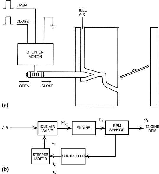
Figure 7.6 Idle speed control system.
There are various schemes for operating a valve to introduce bypass air for idle control. One relatively common method for controlling the idle speed bypass air uses a special type of motor called a stepper motor. One stepper motor configuration consists of a rotor with permanent magnets and two sets of windings in the stator that are powered by separate driver circuits. The configuration of a stepper motor is similar to that of a brushless DC motor as explained in Chapter 6 (see Figure 6.36). Such a motor can be operated in either direction by supplying pulses in the proper phase to the windings as explained in Chapter 6. This is advantageous for idle speed control since the controller can very precisely position the idle bypass valve by sending the proper number of pulses of the correct phasing.
A digital engine control computer can precisely determine the position of the valve in a number of ways. In one way, the computer can send sufficient pulses to close completely the valve when the ignition is first switched on. Then it can open pulses (phased to open the valve) to a specified (known) position. The physical configuration for the idle speed control is depicted in Figure 7.6a. The variables have the same notation as given in Chapter 5.
In addition, the digital engine control system receives digital on/off status inputs from several power-consuming devices attached to the engine, such as the air conditioner clutch switch, park-neutral switch, and the battery charge indicator. These inputs indicate the load that is applied to the engine during idle.
Discrete Time Idle Speed Control
In Chapter 5, an idle speed control system (ISC) was introduced based upon the continuous time control theory of Chapter 1. As explained in Chapter 5, the purpose of the ISC is to maintain the engine idle speed Ω at a constant (set point) value Ωs. The ISC is one of many control modes of the digital engine control system. Since this function is implemented digitally, the ISC is inherently a discrete time system.
In this section, we consider a digital (i.e., discrete time) implementation of the same ISC that was presented in Chapter 5. Figure 7.7 is a block diagram of this discrete time system in which the control subsystem labeled Hc is implemented in the integrated digital electronic engine control system.
Figure 7.7 Discrete time idle speed control block diagram.
The present discussion is an example of discrete time control introduced in Chapter 2. In this figure, the plant being controlled consists of the engine with the idle air bypass actuator. This plant is an analog system modeled by continuous time equations. Using the Laplace transform methods of Chapter 1, it was shown in Chapter 5, that, for the example ISC, the plant transfer function Hp(s) is given by
![]() (25)
(25)
The desired idle angular speed (or set point for the controller) is denoted Ωs in Figure 7.7. Also depicted in the block diagram of this figure is the actual idle angular speed Ω(t) or Ω(s). A measurement of Ω made by the sensor is fed back to the system input forming an error ![]() :
:
![]() (26)
(26)
In the example of Chapter 5 it was assumed for computational simplicity that the sensor is ideal such that Hs(s) = 1. For the purposes of comparing the continuous time idle speed control system with the present discrete time, digital implementation we make the same assumption here along with assuming the same plant model.
In the present discrete time implementation, the error is sampled periodically with period T. In accordance with the discrete time control theory of Chapter 2 we assume an ideal sampler/quantizer (i.e. A/D converter) such that the input to the discrete time control system is ![]() :
:
![]() (27)
(27)
We further assume that in keeping with the continuous time system, the control is PI. The continuous time model for the control system is given by its operational transfer function:
 (28)
(28)
In the time domain, the control variable u(t) can be written as
The discrete time model for u(t) at sample time tk(i.e., uk) is given by
![]()
In the PI model ukI is the discrete time version of the integral term evaluated at time tk. There are many ways of approximating the continuous time integral with a discrete time version. The trapezoidal integration rule is chosen here. In this method, the integral of ![]() at time tk can be approximated by the following:
at time tk can be approximated by the following:
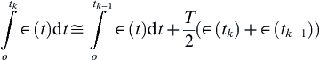 (29)
(29)
where the second term approximates the contributions to the integral at tk by the integral evaluated at tk−1 + the area of a trapezoidal area under the function ![]() from tk−1 to tk. Using this model, we obtain the following recursive equation:
from tk−1 to tk. Using this model, we obtain the following recursive equation:
![]() (30)
(30)
Taking the z-transform of this equation yields the following expression:
![]() (31)
(31)
This equation can be rewritten as
![]() (32)
(32)
It can be shown that the z-transform operational transfer function Hc(z) is given by
 (33)
(33)
The controller outputs a sequence {uk} control signal that is converted to a piecewise continuous time control signal ![]() via the ZOH (see Chapter 2) which operates the plant actuator.
via the ZOH (see Chapter 2) which operates the plant actuator.
It was also shown in Chapter 2 that the z-transform operational transfer function of the combination ZOH and plant G(z) is given by
![]() (34)
(34)
As shown in Chapter 2 the method of finding the z-transform of Hp(s)/s is first to find the partial fraction expansion of this function and then using the table of Chapter 2 to find the individual z-transforms of each partial fraction. Then the desired G(z) is found by combining those terms into a ratio of polynomials in z. It can be shown using this procedure that G(z) for the example system with sample time T = 0.01 s is given by
![]()
The z-transform operational transfer function for the forward path HF(z) is given by
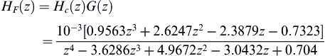 (35)
(35)
The closed-loop transfer function HCL(z) (as explained in Chapter 2) is given by
![]() (36)
(36)
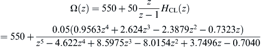
It can be shown that, using the parameters of the example of Chapter 5, HCL(z) is given by
![]() (37)
(37)
The four poles of HCL(z) are given by
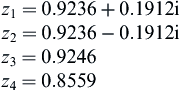
All four poles are inside the unit circle (|z| = 1) in the complex z-plane so the system is stable.
In Chapter 5, the performance of the continuous time ISC was examined by computing the step response in which the command speed was changed from 550 to 600 RPM at time t = 0.5 s. A similar step change can be determined for the discrete time ISC by assuming a command input ΩS(t) given by
![]() (38)
(38)
where u(t) = unit step at t = 0. The z-transform of the ISC dynamic response to this input is given by
 (39)
(39)
The system output at times tk can be found by writing the partial fraction expansion for the product y(z):
![]() (40)
(40)
As shown in Chapter 2 this partial fraction is of the form

where αm is the residue of y(z) at pole zm and zm denotes poles of y(z) m=1,2,3,4,5.
The response of the system at time tk which is denoted yk was shown in Chapter 2 (by equating coefficients of z−k on both sides of the above equation) to be given by
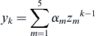
Figure 7.8 is a plot of Ω(tk) where
![]()

Figure 7.8 Step response of discrete time idle speed control.
A comparison of Figure 5.29 in Chapter 5 with Figure 7.8 shows that the dynamic performance of the discrete time digital version of ISC is nearly identical with the corresponding continuous time system. When the engine is not idling, the idle speed control valve may be completely closed so that the throttle plate has total control of intake air.
EGR Control
A second electronic engine control subsystem involves the control of exhaust gas that is recirculated back to the intake manifold. Under normal operating conditions, engine cylinder temperatures can reach a point at which NOx is formed during combustion. The exhaust will have NOx emissions that increase with increasing combustion temperature. As explained in Chapter 5, a small amount of exhaust is introduced into the cylinder to replace some of the normal intake air. This results in lower combustion temperatures, which reduces NOx emissions.
The control mode selection logic determines when EGR is turned off or on. EGR is turned off during cranking, cold engine temperature (engine warm-up), idling, acceleration, or other conditions demanding high torque. Since exhaust gas recirculation was first introduced as a concept for reducing NOx exhaust emissions, its implementation has gone through considerable change. There are, in fact, many schemes and configurations for EGR realization. We discuss here one method of EGR implementation that incorporates enough features to be representative of all schemes in use today and in the near future.
Fundamental to all EGR schemes is a passageway or port connecting the exhaust and intake manifolds. A valve is positioned along this passageway whose position regulates EGR from zero to some maximum value. In one configuration, the valve is operated by a diaphragm connected to a variable vacuum source. The controller operates a solenoid in a periodic variable-duty-cycle mode. By varying this duty cycle, the control system has proportional control over the EGR valve opening and thereby over the amount of EGR. However, EGR activation also can be done using a motor such as a stepper motor as described in Chapter 6. The solenoid-based EGR actuator has cost advantages over a motor-based system, although manifold vacuum required to operate it varies with engine-operating conditions and is very low at wide open throttle.
In many EGR control systems the controller monitors the differential pressure between the exhaust and intake manifold via a differential pressure sensor (DPS). With the signal from this sensor, the controller can calculate the valve opening for the desired EGR level. The amount of EGR required is a predetermined function of the load on the engine (i.e., power produced).
A simplified block diagram for an exemplary EGR control system is depicted in Figure 7.9. In this figure, the EGR valve is operated by a solenoid-regulated vacuum actuator (coming from the intake). An explanation of this proportional actuator is given in Chapter 6. The engine controller determines the required amount of EGR based on the engine-operating condition and the signal from the differential pressure sensor (DPS) between intake and exhaust manifolds. The controller then commands the correct EGR valve position to achieve the desired amount of EGR via a variable-duty-cycle actuator signal.

Figure 7.9 EGR control block diagram.
The optimum amount of EGR can be determined empirically as a function of engine-operating conditions. Ideally, closed-loop control of EGR would require, for example, a combustion temperature sensor. Although a cost-effective sensor for directly measuring combustion temperature has not been developed yet, there is a correlation between exhaust gas temperature and combustion temperature. The former is readily measurable with relatively inexpensive sensors. In principle, the amount of EGR could be based upon a closed-loop control system using exhaust gas temperature measurements for a feedback signal.
Variable Valve Timing Control
Chapter 5 introduced the concept and relative benefits of variable valve timing for improved volumetric efficiency. There it was explained that performance improvement and emission reductions could be achieved if the opening and closing times (and ideally the valve lift) of both intake and exhaust valves could be controlled as a function of operating conditions. In Chapter 6, a representative mechanism was discussed for varying camshaft phasing that can be used for varying either/both intake and exhaust camshaft phasing. This system improves volumetric efficiency by varying valve overlap from exhaust closing to intake opening as well as the absolute phase of valve opening and closing. In addition to improving volumetric efficiency, this variable valve phasing can assist in achieving desired EGR fraction.
The amount of valve overlap is directly related to the relative exhaust–intake camshaft phasing. Generally, minimal overlap is desired at idle. The desired optimal amount of overlap is determined during engine development as a function of RPM and load (e.g., by engine mapping).
The desired exhaust and/or intake camshaft phasing is stored in memory (ROM) in the engine control system as a function of RPM and load. Then during engine operation the correct camshaft phasing can be found via table lookup and interpolation based on measurements of RPM and load. The RPM measurement is achieved using a noncontacting angular speed sensor (see Chapter 6). Load is measured either using MAF as well as RPM or via an MAP sensor (see Chapter 6).
Once the desired camshaft phasing has been determined, the engine control system sends an appropriate electrical control signal to an actuator (e.g., a motor or a solenoid-operated valve). In Chapter 5, it was shown that for one configuration camshaft phasing is regulated by the axial position of a helical spline gear. This axial position is determined by the pressure of (engine) oil action on one face of the helical spline gear acting against a spring. This oil pressure is regulated by the solenoid-operated valve.
In Chapter 6, an alternate mechanism for varying camshaft phasing is implemented using oil pressure-activated movable vanes in recesses in the camshaft drive gear. For either this latter mechanism or one based upon a helical gear axial position, closed-loop control enables the engine control system to optimize volumetric efficiency.
Since a variable valve phasing system is in fact a position control system, closed-loop control of a camshaft phase requires a measurement of camshaft position relative to the crankshaft. This angular position measurement can be accomplished by measuring the angle between the camshaft and its drive gear. Numerous angular-position sensor configurations are discussed in Chapter 6. For the following discussion of VVP, it is assumed that such a sensor is part of the system. Figure 7.10a depicts a physical configuration of a representative camshaft phasing control system.
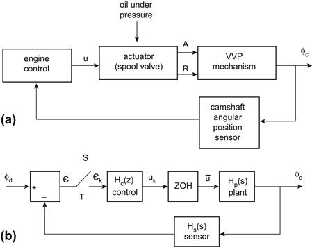
Figure 7.10 Physical configuration and block diagram of VVP system.
Control of a variable valve phasing (VVP) mechanism has a number of objectives and is subject to certain constraints based upon automotive engine-operating characteristics. Except for steady highway cruise, an automotive engine load and RPM vary over a relatively large range. Consequently, the VVP control must have the capability to follow relatively rapid changes in command. The response to step changes in command should have relatively low overshoot (e.g., <10%) and should reach its command position without a steady-state offset. The control, of course, must be stable, and should be robust with respect to parameter changes. The example VVP system presented here is based upon the actuation mechanism described in Chapter 6 which uses vanes attached to the camshaft that move within recesses in the camshaft drive gear. Recall that movement of the vanes relative to this gear results in the variation in camshaft phasing. Recall also that movement of the vanes within the gear recesses is in response to differential pressure on opposite sides of each vane, resulting from a spool valve actuator, which supplies engine oil under pressure to A or R chambers as shown in Figure 7.10a. The dynamic response of the VVP control system should be robust with respect to oil viscosity, which changes with changes in engine temperature; that is, the closed-loop gain for the control system should have large gain and phase margins (see Chapter 1).
The VVP control is one function of the digital control system. When operating in VVP mode the block diagram of the VVP is shown in Figure 7.10b. As explained in Chapter 2, a discrete time control system that regulates a continuous time plant requires a sample and A/D converter as well as a zero order hold (ZOH), both of which are incorporated in the block diagram of Figure 7.10b. Sensor measurements for such a system are assumed to be ideal such that the sensor transfer function is taken to be
![]()
In Chapter 6, it was shown that the plant transfer function for this VVP configuration is given by
![]() (41)
(41)
For the present example, the following parameters are chosen:
![]()
A PID control law is selected to provide sufficient flexibility to meet design objectives. The continuous time PID control law is given by
![]() (42)
(42)
Using the root locus techniques of Chapter 1, the following gain parameters are given which satisfy the overshoot and response time criteria:
One of the requirements for the VVP control system is robust stability; in Chapter 1, it was shown that robustness is expressed meaningfully by gain and phase margins as determined by the bode plot for the product Hc(s)Hp(s). Figure 7.11 is the Bode plot for this system.

Figure 7.11 Bode plot of HF(s) for VVP system.
The gain crossover frequency is at 10 rad/s and the phase margin there is about 109 degrees. The phase crossover frequency is at about .02 rad/sec where the gain margin is more than 100 dB. This system has very robust stability.
The discrete time model for the control system is given by
![]() (43)
(43)
In the section on idle speed control, it was shown that the z-transform of ukI using trapezoidal integration rule is given by
Combining all three terms in the control variable uk of Eqn (37), the control system transfer function Hc(z) is given by
 (44)
(44)
The plant and ZOH z-transform operational transfer function G(z) is found using the method given in Chapter 2:
![]()
The z-transform in the above equation can be found by expanding Hp(s)/s in a partial fraction. The function ![]() is given by
is given by
![]() (45)
(45)
This function has a double pole at s = 0. Using the parameters for the plant given above, the partial fraction expansion is given by
![]() (46)
(46)
Using the tables of z-transforms from Chapter 2 and assuming a sample period T = 0.01 sec, the operational transfer function G(z) is given by
 (47)
(47)
where ![]()
The poles of G(z) are all on or in the unit circle which assures a stable system with a combined transfer function:
![]() (48)
(48)
Using the gain parameters Kp, KD, and KI given above, the forward transfer function HF (from ![]() to the plant output
to the plant output ![]() ) is given by
) is given by
 (49)
(49)
The closed-loop z-transfer function Hcl(z) is given by
![]() (50)
(50)
![]()
![]() (51)
(51)
The poles of the closed-loop transfer function are given by
All poles are within the unit circle for which system stability is assured.
The dynamic response of the VVP system is illustrated by finding the output sequence ![]() for 10° step command input which is given by
for 10° step command input which is given by
![]()
The z-transform of ![]() is given by
is given by
![]()
The camshaft phase (i.e., system output) is given by
![]()
The output sequence ![]() at time tk is found using the method of finding the inverse z-transform explained in Chapter 2. Recall that this method involves finding the partial fraction expansion of
at time tk is found using the method of finding the inverse z-transform explained in Chapter 2. Recall that this method involves finding the partial fraction expansion of ![]() and writing each term as a power series in z−k. The output camshaft phase
and writing each term as a power series in z−k. The output camshaft phase ![]() at time tk is the sum of all coefficient of z−k in the separate power series terms in the partial fraction expansion.
at time tk is the sum of all coefficient of z−k in the separate power series terms in the partial fraction expansion.
Figure 7.12 is a plot of this sequence vs. time tk: The transient response error has essentially decayed to zero in less than 0.5 sec and the overshoot is 6.5%. Thus, this digital variable camshaft phase control system meets the original objectives.

Figure 7.12 VVP response to 10-degree step command.
Electronic Ignition Control
As explained in Chapter 5, an engine must be provided with fuel and air in correct proportions and the means to ignite this mixture in the form of an electric spark. Before the development of contemporary electronic ignition, the traditional ignition system included spark plugs, a distributor, and a high-voltage ignition coil. The distributor (which was a form of rotary switch) would sequentially connect the coil output high voltage to the correct spark plug. In addition, it would cause the coil to generate the spark by interrupting the primary current (via ignition points) in the coil circuit, thereby generating the required spark. The time of occurrence of this spark (i.e., the ignition timing) in relation of the piston to TDC which influences the torque generated was determined mechanically by distributor phasing relative to the engine cycle.
The distributor and single coil have been replaced by multiple coils and an electronic control system. Each coil supplies the spark to either one or two cylinders. In such a system, the controller selects the appropriate coil and delivers a trigger pulse to the ignition control circuitry at the correct time for each cylinder. (Note: In some cases, the coil is on the spark plug as an integral unit.)
Figure 7.13 illustrates such a system for an example 4-cylinder engine.
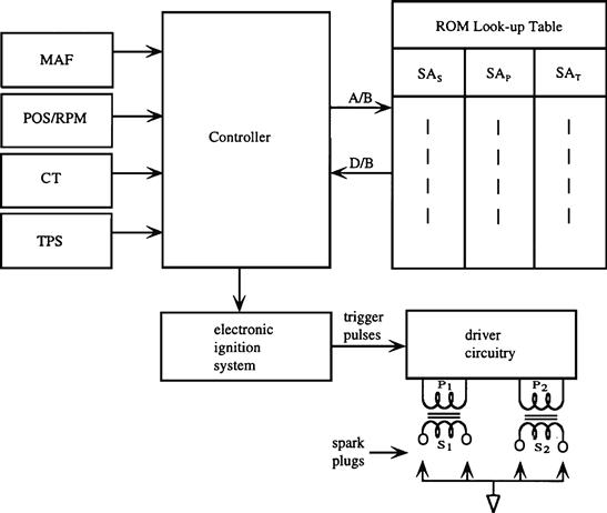
Figure 7.13 Example integrator circuit diagram.
In this example, a pair of coils provides the spark for firing two cylinders for each coil. Cylinder pairs are selected such that one cylinder is on its compression stroke while the other is on exhaust. The cylinder on compression is the cylinder to be fired (at a time somewhat before it reaches TDC). The other cylinder is on exhaust. The coil fires the spark plugs for these two cylinders simultaneously. For the former cylinder, the mixture is ignited and combustion begins for the power stroke that follows. For the other cylinder (on exhaust stroke), the combustion has already taken place and the spark has no effect.
Although the mixture for contemporary vehicle engines is constrained by emissions regulations, the spark timing can be varied in order to achieve optimum performance within the exhaust emission constraint. For example, the ignition timing can be chosen to produce the best possible engine torque for any given operating condition. This optimum ignition timing is known for any given engine configuration from empirical studies of engine performance as measured on an engine dynamometer. As explained in Chapter 5, this optimum ignition timing is known as “spark advance for mean best torque” which is abbreviated MBT.
Ignition timing is normally represented quantitatively by the angular position of the crankshaft relative to TDC for each cylinder during its compression stroke. Spark occurs before TDC because of the time required for combustion to be completed such that power during the power stroke is optimized. Spark timing in degrees of crankshaft rotation is termed “spark advance” (SA).
In the example configuration of Figure 7.13, the spark advance value is computed in the main engine control (i.e., the same controller that regulates fuel). This system receives data from the various sensors (as described above with respect to fuel control) and determines the correct spark advance for the instantaneous operating condition.
The variables that influence the optimum spark timing at any operating condition include RPM, manifold pressure (or mass airflow), barometric pressure, and coolant temperature. The correct ignition timing for each value of these variables is stored in an ROM lookup table. The engine control system obtains readings from the various sensors and generates an address to the lookup table (ROM). After reading the data from the lookup tables, the control system computes the correct spark advance (possibly including interpolation). An output signal is generated at the appropriate time to activate the spark.
In the configuration depicted in Figure 7.13, the electronic ignition is implemented in a stand-alone ignition module. This solid-state module receives the correct spark advance data and generates electrical signals that operate the coil driver circuitry. These signals are produced in response to timing inputs coming from crankshaft and camshaft signals (POS/RPM).
The coil driver circuits generate the primary current in windings P1 and P2 of the coil packs depicted in Figure 7.13. These primary currents build up during the so-called dwell period before the spark is to occur. The process of spark generating for ignition purposes was explained in Chapter 6. There it was explained that the spark is produced by a short-duration very high voltage that is generated in the ignition coil. In the example depicted in Figure 7.13, a pair of coil packs, each firing two spark plugs, is shown. Such a configuration would be appropriate for a 4-cylinder engine. Normally, there would be one coil pack for each pair of cylinders or possibly for each cylinder.
In a typical electronic ignition control system, the total spark advance, SA (in degrees before TDC), is made up of several components that are added together:
![]() (52)
(52)
The first component, SAS, is the basic spark advance, which is a tabulated function of RPM and MAP or MAF. The control system reads RPM and MAP, or MAF and calculates the address in ROM of the SAS that corresponds to these values. Figure 7.14 depicts a representative variation in SAS vs. RPM.

Figure 7.14 Representative SA curve versus RPM.
In the example, the advance of RPM from idle to about 1200 RPM is relatively slow. Then, from about 1200 to about 2300 RPM the slope of SAs with respect to RPM is relatively steep. Beyond 2300 RPM, the increase in SAs with respect to RPM is again relatively small. Each engine configuration has its own spark advance characteristic, which is normally a compromise between a number of conflicting factors (the details of which are beyond the scope of this book). The SAs tabulated values that are placed in ROM are normally determined via engine mapping during development of an engine control system.
The second component, SAP, is the contribution to spark advance due to mass airflow or manifold pressure. This value is obtained from ROM lookup tables with MAF or MAP as the independent variable. In general, the SAP is reduced as intake manifold pressure increases, owing to an increase in combustion rate with pressure.
The final component, SAT, is the contribution to spark advance due to temperature. Temperature effects on spark advance are relatively complex, including such effects as cold cranking, cold start, warm-up, and fully warmed-up conditions, the details of which are beyond the scope of this book.
Closed-Loop Ignition Timing
The ignition system described in the foregoing is an open-loop system. The major disadvantage of open-loop control is that it cannot automatically compensate for mechanical changes in the system. Closed-loop control of ignition timing is desirable from the standpoint of improving engine performance and maintaining that performance in spite of system changes.
One scheme for closed-loop ignition timing is based on the improvement in performance that is achieved by advancing the ignition timing relative to TDC. For a given RPM and manifold pressure, the variation in torque with spark advance is as depicted in Figure 7.15.
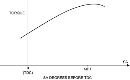
Figure 7.15 Engine brake torque vs. SA.
One can see that advancing the spark relative to TDC increases the torque until a point is reached at which best torque is produced. As introduced above and explained qualitatively in Chapter 5, this spark advance is known as the SA for mean best torque, or MBT.
When the spark is advanced too far, an abnormal combustion phenomenon occurs that is known as knocking. Although the details of what causes knocking are beyond the scope of this book, it is generally a result of a portion of the air–fuel mixture abruptly igniting (autoigniting), as opposed to being normally ignited by the advancing flame front that occurs in normal combustion following spark ignition. Roughly speaking, the amplitude of knock is proportional to the fraction of the total air and fuel mixture that autoignites. It is characterized by an abnormally rapid rise in cylinder pressure during combustion, followed by very rapid oscillations in cylinder pressure. The frequency of these oscillations is specific to a given engine configuration and is typically in the range of a few kilohertz. Figure 7.16 is a graph of a representative cylinder pressure versus time under knocking conditions. A relatively low level of knock is arguably beneficial to performance, although excessive knock is unquestionably damaging to the engine and must be avoided.

Figure 7.16 Cylinder pressure under knock conditions.
One control strategy for spark advance under closed-loop control is to advance the spark timing until the knock level becomes unacceptable. At this point, the control system reduces the spark advance (retarded spark) until acceptable levels of knock are achieved. Of course, a spark advance control scheme based on limiting the levels of knocking requires a knock sensor such as that explained in Chapter 6. This sensor responds to the acoustical energy in the spectrum of the rapid cylinder pressure oscillations, as shown in Figure 7.16.
Figure 7.17 is a diagram of an exemplary instrumentation system for measuring knock intensity. Output voltage VE of the knock sensor is proportional to the acoustical energy in the engine block at the sensor mounting point. This voltage is sent to a narrow bandpass filter that is tuned to the knock frequency (for the particular engine configuration). The filter output voltage VF is proportional to the amplitude of the knock oscillations, and is thus a “knock signal.” The envelope voltage of these oscillations, Vd, is obtained with a detector circuit which can, for example, be implemented with a rectifier-type circuit which includes a diode and a capacitor (see Chapter 3).

Figure 7.17 Instrumentation for measuring knock intensity.
Following the detector in the circuit of Figure 7.17 of the example knock detection system is an electronic gate that normally blocks Vd for much of the engine cycle but passes it during the portion of the engine cycle for which the knock amplitude is largest (i.e., shortly after TDC). The gate is, in essence, an electronic switch that is normally open, but is closed for a short interval (from 0 to T) following TDC. It is during this interval that the knock signal is largest in relationship to engine noise. The probability of successfully detecting the knock signal is greatest during this interval. Similarly, the possibility of mistaking normal engine acoustic noise for true knock signal is smallest during this interval.
The final stage in the exemplary knock-measuring instrumentation is integration with respect to time. Integration can be accomplished numerically in the engine control or as a part of the knock sensor instrumentation using an operational amplifier circuit configured to perform analog integration. For example, the circuit of Figure 7.18a could be used to integrate the gate output. In our example system, the electronic gate is implemented via a pair of switches S1 and S2. Switch S1 is normally open and S2 closed but S1 is closed and S2 opened at t = 0 corresponding to the beginning of the period where knock can occur. The end of this period is t = T. This gate operation is repetitive and occurs following TDC for the power stroke of the associated cylinder. The output voltage VK at the end of the gate interval T is given by
 (53)
(53)
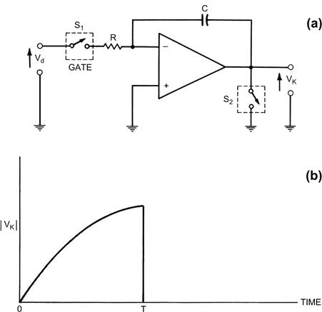
Figure 7.18 Analog integrator for knock detection system.
This voltage increases sharply in magnitude but is negative for Vd as depicted in Figure 7.18b because the input is connected to the op amp inverting input. Figure 7.18b is a plot of the absolute magnitude of Vk (i.e., |Vk|). This voltage reaches a maximum amplitude at the end of the gate interval, as shown in Figure 7.18b, provided knock occurs. However, if there is no knock, VK remains near zero.
The level of knock intensity is indicated by voltage |VK(T)| at the end of the gate interval. The spark control system compares this voltage with a threshold voltage to determine whether knock has or has not occurred.
This envelope-detected voltage is sent to the controller, where it is compared with a level corresponding to the knock intensity threshold. Whenever the knock level is less than the threshold, the spark is advanced. Whenever it exceeds the threshold, the spark is retarded. The comparator function is normally implemented in the digital control system by numerically comparing the integrated knock intensity signal with a threshold TK (under program control; see Figure 7.19).
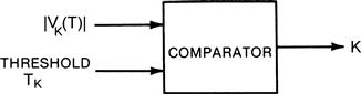
Figure 7.19 Comparator for knock detector.
In such an implementation, the controller generates a binary-valued variable (denoted K in Figure 7.19) having the following algorithm:
![]() (54)
(54)
Knock detection with the above algorithm has two types of error: (1) missed detection in which knock has occurred but the system output is K = 0 and (2) false alarm in which there is normal combustion but the system output is K = 1. The quantitative error analysis for the above knock detection method generally is covered in the field of statistical decision theory. The theory of this topic is outside the scope of this book. However, for those readers having a background in statistical analysis, we present the following brief models and analysis of the probability of error in the above knock detection system.
Essentially, the voltage of any point in the exemplary knock detection system is a random process. In this exemplary knock detection system, the detection of knock is based upon the voltage VK(T) and is, in effect, a form of statistical hypothesis testing. This method can perhaps best be explained from the histogram of Figure 7.20 for voltage VK(T) for a large sample of engine cycles under the two hypotheses:

Figure 7.20 Histogram for hypotheses H0 and H1.
For notational convenience, we let x = |VK(T)| in Figure 7.20. In this figure, the number of occurrences of x at a particular value for hypothesis H0 is denoted ![]() and for hypothesis H1 is denoted
and for hypothesis H1 is denoted ![]() . For a sufficiently large sample space, these histograms approach the continuous probability density functions for the two hypotheses that are denoted
. For a sufficiently large sample space, these histograms approach the continuous probability density functions for the two hypotheses that are denoted ![]() and
and ![]() , respectively.
, respectively.
The detection threshold TK is depicted in Figure 7.20. The total probability of error Pe for our example knock detection method is given by
 (55)
(55)
where the first term corresponds to false alarm errors and the second to missed detection errors. For any such knock detection method, an optimum threshold that minimizes the total probability of error can be determined empirically.
Although this scheme for knock detection has shown a constant threshold, there are some production applications that have a variable threshold. The threshold in such cases increases with RPM because the competing acoustical noises in the engine increase with RPM.
Spark Advance Correction Scheme
Although the details of spark advance control vary from manufacturer to manufacturer, there are generally two classes of correction that are used: fast correction and slow correction. In the fast correction scheme, the spark advance is decreased for the next engine cycle by a fixed amount (e.g., 5°) whenever knock is detected. Then the spark advance is incremented in one-degree increments every 5–20 crankshaft revolutions.
The fast correction ensures that minimum time is spent under heavy knocking conditions. Further, this scheme compensates for hysteresis (i.e., for one degree of spark advance to cause knocking, more than one degree must be removed to eliminate knocking). The fast correction scheme is depicted qualitatively by the waveform depicted in Figure 7.21.

Figure 7.21 Fast correction of SA.
In the slow correction scheme (Figure 7.22), spark advance is decreased by one (or more) degree each time knock is detected, until no knocking is detected. The spark advance proceeds in one-degree increments after many engine cycles.
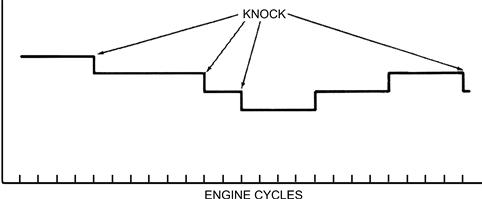
Figure 7.22 Slow correction of SA.
The slow correction scheme is more of an adaptive closed-loop control than is the fast correction scheme. It primarily is employed to compensate for relatively slow changes in engine condition or fuel quality (i.e., octane rating).
Integrated Engine Control System
Each control subsystem for fuel control, spark control, and EGR has been discussed separately. However, in a contemporary vehicle an integrated electronic engine control system employs an open architecture and can include these subsystems and provide additional functions. (Usually, the flexibility of the digital control system allows such expansion quite easily because the computer program can be changed to accomplish the expanded functions.) Several of these additional functions are discussed in the following.
Secondary Air Management
Secondary air management is used to improve the performance of the catalytic converter by providing extra (oxygen-rich) air either to the converter itself or to the exhaust manifold. The catalyst temperature must be above about 200 °C to efficiently oxidize HC and CO and reduce NOx. During engine warm-up when the catalytic converter could be cold, HC and CO are oxidized in the exhaust manifold by routing secondary air to the manifold. This creates extra heat to speed warm-up of the converter and EGO sensor, enabling the fuel controller to go to the closed-loop mode relatively quickly.
The converter can be damaged if too much heat is applied to it. This can occur if large amounts of HC and CO are oxidized in the manifold during periods of heavy loads, which call for fuel enrichment, or during severe deceleration. In such cases, the secondary air is directed to the air cleaner, where it has no effect on exhaust temperatures.
After warm-up, the main use of secondary air is to provide an oxygen-rich atmosphere in the second chamber of the three-way catalyst, dual-chamber converter system. In a dual-chamber converter, the first chamber contains rhodium, palladium, and platinum to reduce NOx and to oxidize HC and CO. The second chamber contains only platinum and palladium. The extra oxygen from the secondary air improves the latter converter’s ability to oxidize HC and CO in the second converter chamber.
The computer program for the control mode selection logic can be modified to include the conditions for controlling secondary air. In one configuration, the engine controller regulates the secondary air by using two solenoid valves similar to the EGR valve. One valve switches airflow to the air cleaner or to the exhaust system. The other valve switches airflow to the exhaust manifold or to the converter. The air routing is based on engine coolant temperature and air/fuel ratio. The control system diagram for secondary air is shown in Figure 7.23.
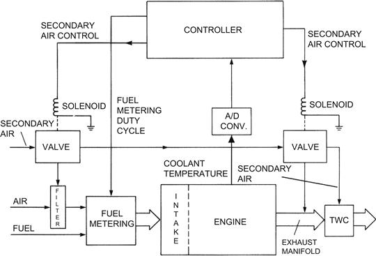
Figure 7.23 Secondary air system.
Evaporative Emissions Canister Purge
In pre-emission controlled vehicles, the fuel stored in the fuel system tended to evaporate and release hydrocarbons (HCs) into the atmosphere. In contemporary vehicles, to reduce these HC emissions, the fuel tank is sealed and evaporative gases are collected by a charcoal filter in a canister. The collected fuel is released into the intake through a solenoid valve controlled by the computer. This normally is done during closed-loop operation to reduce fuel calculation complications in the open-loop mode.
Automatic System Adjustment
Another important feature of microcomputer engine control systems is their ability to be programmed to adapt to parameter changes. Many control systems use this feature to enable the computer to modify lookup table values for computing open-loop air/fuel ratios. While the computer is in the closed-loop mode, the computer checks its open-loop calculated air/fuel ratios and compares them with the closed-loop average limit cycle values. If they match closely, the open-loop lookup tables are unchanged. If the difference is large, the system controller corrects the lookup tables so that the open-loop values more closely match the closed-loop values. This updated open-loop lookup table is stored in separate memory (RAM), which is always powered directly by a car battery or a separate “keep alive” battery so that the new values are not lost while the ignition key is turned off. The next time the engine is started, the new lookup table values will be used in the open-loop mode and will provide more accurate control of the air/fuel ratio than the unmodified values. This feature is very important because it allows the system controller to adjust to long-term changes in engine and fuel system conditions. This feature can be applied in individual subsystem control systems or in the fully integrated control system. If not available initially, it may be added to the system by modifying its control program.
System Diagnosis
Another important feature of microcomputer engine control systems is their ability to diagnose failures in their control systems or components and alert the operator. Sensor and actuator failures or misadjustments can be detected readily by the computer under certain operating conditions. For instance, the computer will detect a malfunctioning MAF sensor if the sensor’s output goes above or below certain specified limits, or fails to change for long periods of time. A prime example is the automatic adjustment system just discussed. If the open-loop calculations consistently come up different from those indicated in closed-loop mode, the engine control computer may determine that one of the many sensors used in the open-loop calculations has experienced a calibration change or has failed completely.
If the computer detects the loss of a primary control sensor or actuator, it may switch to in a different mode until the problem is repaired. The operator is notified of a failure by an indicator on the instrument panel (e.g., check engine indicator). Because of the flexibility of the microcomputer engine control system, additional diagnostic programs might be added to accommodate different engine models that contain more or fewer sensors. Keeping the system totally integrated gives the microcomputer controller access to more sensor inputs so they can be checked. Chapter 10 discusses system diagnosis in detail. Often, there is sufficient redundancy to permit suboptimal engine operation when a component has failed such that the vehicle can be driven to a repair facility in an operating mode that has been termed a “limp home mode.”
Summary of Control Modes
A summary of the control modes for a digital engine control system is presented below.
Engine Crank (Start)
The following list is a summary of the engine operations in the engine crank (starting) mode, wherein the primary control concern is rapid and reliable engine start:
Engine Warm-Up
While the engine is warming up, the engine temperature is rising to its normal operating value. Here, the primary control concern is rapid and smooth engine warm-up. A summary of the engine operations during this period is as follows:
1. engine RPM above cranking speed at command of driver,
2. engine coolant temperature rises to minimum threshold,
4. spark timing set by controller,
7. secondary air to exhaust manifold,
8. fuel economy not as closely controlled as fully warmed engine, and
9. emissions not as closely controlled as fully warmed engine.
Open-Loop Control
The following list summarizes the engine operations when the engine is being controlled in an open-loop mode. This mode is used before the EGO sensor has reached the correct temperature for closed-loop operation. Fuel economy and emissions are closely controlled.
Closed-Loop Control
For the closest control of emissions and fuel economy under various driving conditions, the electronic engine control system is in a closed loop. Fuel economy and emissions are controlled very tightly. The following is a summary of the engine operations during this period:
1. engine RPM at command of driver (or idle speed control),
2. engine temperature in normal range (above warm-up threshold),
3. average air/fuel ratio controlled to 14.7, ±0.05,
4. EGO sensor’s temperature above minimum threshold detected by a sensor output voltage indicating a rich mixture of air and fuel for a minimum amount of time,
5. system returns to open loop if EGO sensor cools below minimum threshold or fails to indicate rich mixture for given length of time,
7. secondary air to catalytic converter,
Hard Acceleration
When the engine must be accelerated quickly or if the engine is under heavy load, it is in a special mode. Now, the engine controller is primarily concerned with providing maximum performance. Here is a summary of the operations under these conditions:
1. driver asking for sharp increase in RPM or in engine power (via rapid throttle angle increase), demanding maximum torque,
2. engine temperature in normal range,
3. air/fuel ratio rich mixture,
4. EGO not in loop (very briefly),
7. relatively poor fuel economy (relative to normal closed loop), and
8. relatively poor emissions control (relative to normal closed loop).
Deceleration and Idle
Slowing down, stopping, and idling are combined in another special mode. The engine controller is primarily concerned with reducing excess emissions during deceleration, and keeping idle fuel consumption at a minimum. This engine operation is summarized in the following list:
1. RPM decreasing rapidly due to driver command or else held constant at idle,
2. engine temperature in normal range,
3. air/fuel ratio lean mixture,
4. special mode in deceleration to reduce emissions,
5. special mode in idle to keep RPM constant at idle as load varies due to air conditioner, automatic transmission engagement, etc.,
8. good fuel economy during deceleration, and
9. possibly relatively poor fuel economy during idle, but fuel consumption kept to minimum possible (except for hybrid electric vehicle (HEV)).
Automatic Transmission Control
The vast majority of cars and light trucks sold in the United States are equipped with automatic transmissions. The majority of these transmissions are controlled electronically. The configuration of an automatic transmission consists of a torque converter and a sequence of planetary gear sets.
The transmission (whether automatic or manual) is a gear system that adjusts the ratio of engine speed to wheel speed. Essentially, the transmission enables the engine to operate within its optimal performance range regardless of the vehicle load or speed. It provides a gear ratio between the engine speed and vehicle speed such that the engine provides adequate power to drive the vehicle at any speed. Any gear system connecting a pair of shafts along which torque/power is transmitted is the mechanical equivalent of an electrical transformer. Just as a transformer can maximize the power transmitted from a source to a load, a gear system has the capability of maximizing the transfer of engine power to the load at the drive wheels while maintaining engine speed (under load) at acceptable values.
To accomplish optimal power transfer to the load with a manual transmission, the driver selects the correct gear ratio from a set of possible gear ratios (usually three to five for passenger cars). An automatic transmission selects the gear ratio by means of an automatic control system.
The configuration for an automatic transmission consists of a fluid-coupling mechanism, known as a torque converter, and a system of planetary gear sets. The torque converter is formed from a pair of structures of a semitoroidal shape (i.e., a donut-shaped object split along the plane of symmetry). Figure 7.24 is a schematic sketch of a torque converter showing the two semitoroids.
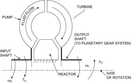
Figure 7.24 Torque converter configuration.
One of the toroids is driven by the engine by the input shaft and is called the pump. The other is in close proximity and is called the turbine. Both the pump and the turbine have vanes that are nearly in axial planes. In addition, a series of vanes are fixed to the frame and are called the reactor. The entire structure is mounted in a fluid-tight chamber and is filled with a hydraulic fluid (i.e., transmission fluid). As the pump is rotated by the engine, the hydraulic fluid circulates as depicted by the arrows in Figure 7.24. The fluid impinges on the turbine blades, imparting a torque to it. The torque converter provides a fluid coupling to transmit engine torque and power to the turbine from the engine. The torque that is applied to the pump portion of the torque converter is the engine brake torque (Tb). Denoting the torque applied to the output shaft by the turbine TT, this latter torque is given by TT = TRTb where TR is the torque multiplication factor of the torque converter. However, the properties of the torque converter are such that when the vehicle is stopped corresponding to a nonmoving turbine, the engine can continue to rotate (as is does when the vehicle is stopped with the engine running). Normally, with the vehicle stopped and the torque converter output shaft not rotating, the engine is at idle and producing minimal Tb. The turbine blades are in a stalled condition and TT is sufficiently low that only a small torque applied to the wheels by the brakes is capable of stopping the vehicle.
A detailed analytical model for a torque converter is given in a paper by Allen Kotwicki.∗ In this paper, it is explained that a torque converter is a form of fluid coupling device in which a reactor is added which is rigidly connected to the transmission housing and normally does not rotate. However, torque converter efficiency is improved whenever the torque reaction on the fluid is zero by allowing the reactor to rotate freely. The torque converter is filled with transmission fluid that is caused to circulate through the pump–turbine–reactor by rotation of the pump by the engine crankshaft rotation. This fluid flows in an annular path as depicted in Figure 7.24. The operating physical principle upon which a fluid coupling or a torque converter is based is that torque in any such system results from a time rate of change of angular momentum. In the reference cited above it is shown that the torques of the pump Tp and turbine Tt are given by
![]() (56)
(56)
where ωp = the pump angular speed (rad/s),
where ρ is the transmission fluid density.
In these equations a double subscript on a variable means: first subscript p → pump, r → reactor, t → turbine and the second subscript e → entrance, x → exit. The double-subscripted parameters have the following meaning:
A is the converter cross-sectional area normal to annular flow (p),
It is further shown that the volume flow rate is given by
 (57)
(57)
where E, F, G, H, and I are constants given in the cited reference. In this reference empirical evaluation of coefficients for a first-order linear regression-based polynomial for Q of the form is developed:
![]()
where
![]()
where S is the speed ratio.
Using this approximation, it is shown in the reference that the torque ratio TR is given by
![]() (58)
(58)
where

This simplified model is shown in the reference to correlate well with experimental data and is normally sufficient for development of transmission controls.
The planetary gear system consists of a set of three types of gears connected together as depicted in Figure 7.25a. The inner gear is known as the sun gear. There are three gears meshed with the same gear at equal angles, which are known as planetary gears. These three gears are tied together with a cage that supports their axles. The third gear, known as a ring gear, is a section of a cylinder with the gear teeth on the inside. The ring gear meshes with the three planetary gears.
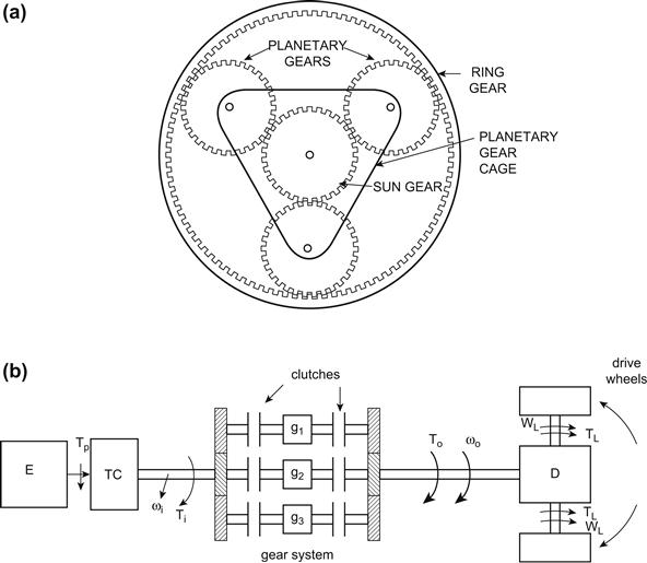
Figure 7.25 Schematic automatic transmission configuration.
In operation, one or more of these gear systems are held fixed to the transmission housing via a set of hydraulically actuated clutches. The action of the planetary gear system is determined by which set or sets of clutches are activated. For example, if the ring gear is held fixed and input power (torque) is applied to the sun gear, the planetary gears rotate in the same direction as the sun gear but at an increased torque. We denote the input torque applied to the sun gear and the angular speed of the shaft driving this gear system by Ti and ωi, respectively. The output torque and its speed are denoted To and ωo, respectively. A model for this gear system is given by
![]() (59)
(59)
![]()
Ns is the number of teeth on the sun gear and Np is the number of teeth on a planetary gear.
If the planetary gear cage is fixed, then the sun gear drives the ring gear in the opposite direction as is done when the transmission is in reverse. If all three sets of gears are held fixed to each other rather than the transmission housing, then direct drive (gear ratio = 1) is achieved.
A typical automatic transmission has a number of planetary gear systems (denoted g1, g2, g3 in Figure 7.25b), each with its own set of hydraulically actuated clutches as depicted schematically in Figure 7.25b. In an electronically controlled automatic transmission, the clutches are electrically or electrohydraulically actuated via solenoid type actuators such as are described in Chapter 6.
Most automatic transmissions have three forward gear ratios, although a few have two and some have four or more and all have reverse. A properly used manual transmission normally has efficiency advantages over an automatic transmission (because of power losses in the torque converter), but the automatic transmission is the most commonly used transmission for passenger automobiles in the United States. In the past, automatic transmissions have been controlled by a hydraulic and pneumatic system, but it is common in contemporary vehicles to use electronic controls as part of an integrated powertrain control system. The control system must determine the correct gear ratio by sensing the driver-selected command, accelerator pedal position, engine load, and vehicle motion. Once again, as in the case of electronic engine control, the electronic transmission control can optimize transmission control. However, since the engine and transmission function together as a power-producing unit, it is sensible to control both components in a single electronic controller. The proper gear ratio is actually computed in the electronic transmission control portion of the powertrain control system.
Figure 7.25b depicts schematically the powertrain denoting the engine E, the torque converter (TC), the gear system, the differential D (having gear ratio gD), and the axles with the drive wheels (which could be front or rear). The configuration and operating principles of the differential are explained later in this chapter. For simplicity, it is convenient to assume that both right and left drive wheels (or all four drive wheels for four-wheel drive) are identical and present a combined load torque TL to the drive axle. In this case, the transmission output torque To is given by
![]()
The gear system consists of a set of planetary gear units each having a gear ratio gn (n = 1,2…N). The appropriate gear is selected by the control system, which operates the correct set of clutches via an electrohydraulic actuator (e.g. solenoid-operated valve supplying transmission fluid under pressure to a set of sprag clutches). For gear systems connected in series, the total gear ratio g from the torque converter output to the load is given by
![]() (60)
(60)
Otherwise, for a parallel connected system of gears as shown in Figure 7.25b, the gear ratio is given by
![]() (61)
(61)
Although there are many possible powertrain control modes depending upon vehicle operating conditions and driver command, an illustrative example mode is maximizing the power delivered to the load (drive wheels) for a given engine brake power (Pb = Tbωe). For example, under certain powertrain operating conditions, the gear ratio, which maximizes this transfer of engine power to load power (PL = TLωL) g,∗ is given approximately by

The controller selects the nearest available gear ratio from the set of possible choices.
Another control mode for the transmission is to maximize drive axle torque TL, thereby maximizing vehicle acceleration whenever the driver command yields wide open throttle (WOT). This mode calls for the maximum available gear ratio subject to the constraint that engine RPM remains near the point for maximum brake torque.
The relevant clutches are activated by the pressure of transmission fluid acting on piston-like mechanisms. The pressure is switched on at the appropriate clutch via solenoid-activated valves that are supplied with automatic transmission fluid under pressure. The solenoids are actuators that receive an electrical signal from the powertrain control system as explained in Chapter 6.
During normal driving, the electronic transmission controller determines the desired gear ratio from measurements of engine load and RPM as well as transmission output shaft RPM. These RPM measurements are made using noncontacting angular speed sensors (usually magnetic in nature) as explained in Chapter 6. Once this desired gear ratio is determined, the set of clutches to be activated is uniquely determined, and control signals are sent to the appropriate clutches.
Normally, the highest gear ratio (i.e., ratio of input shaft speed to output shaft speed) is desired when the vehicle is at low speed such as in accelerating from a stop. As vehicle speed increases from a stop, a switching level will be reached at which the next lowest gear ratio is selected. This switching (gear-changing) threshold is an increasing function of load as measured by the MAF or MAP sensor.
At times (particularly under steady vehicle speed conditions), the driver demands increasing engine power (e.g., for heavy acceleration). In this case, the controller shifts to a higher gear ratio, resulting in higher acceleration than would be possible in the previous gear setting. At a steady-cruise condition, the transmission gear ratio is unity and the total gear ratio from engine to drive wheels is gD (i.e., differential gear ratio). The functional relationship between gear ratio and operating condition is often termed the “shift schedule,” which is programmed into ROM.
Torque Converter Lock-Up Control
As explained above, automatic transmissions use a hydraulic or fluid coupling to transmit engine power to the wheels. There is some relatively small power loss in the TC such that the fluid coupling is less efficient than the nonslip coupling of a pressure-plate manual clutch used with a manual transmission. Thus, fuel economy is usually lower with an automatic transmission than with a standard transmission. This problem has been partially remedied by placing a clutch functionally similar to a standard pressure-plate clutch inside the torque converter of the automatic transmission and engaging it during periods of steady cruise. This enables the automatic transmission to provide fuel economy near that of a manual transmission and still retain the automatic shifting convenience.
The torque converter locking clutch (TCC) is activated by a lock-up solenoid controlled by the engine control system computer. The computer determines when a period of steady cruise exists from throttle position and vehicle speed changes. It pulls in the locking clutch and keeps it engaged until it senses conditions that call for disengagement. This condition is known as “torque converter lock-up.”
Differential and Traction Control
The transmission output shaft is coupled to the drive axles via the differential. The differential is a necessary component of the drivetrain because the left and right drive wheels turn at different speeds whenever the car moves along a curve (e.g., turning a corner). Whenever a car is executing a turn, the outside drive wheel rotates at a higher angular speed than the inside wheel. The differential achieves this function permitting both wheels to propel the vehicle. Figure 7.26 depicts the configuration for a differential. Unfortunately, wherever there is a large difference between the tire/road friction from left to right, the differential will tend to spin the low friction wheel. An extreme example of this occurs whenever one drive wheel is on ice and the other is on dry road. In this case, the tire on the ice side will spin and the wheel on the dry side will not. Typically, the vehicle will not move in such circumstances.
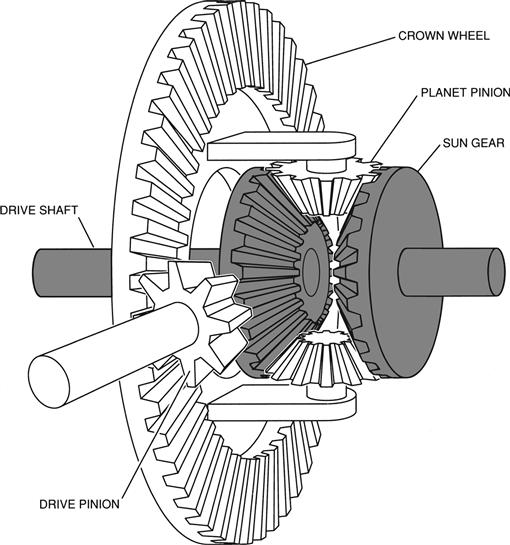
Figure 7.26 Differential configuration.
Certain cars are equipped with so-called traction control devices that can overcome this disadvantage of the differential. Such cars have differentials that incorporate electrohydraulic solenoid-activated clutches somewhat similar to those used in an automatic transmission that can “lock” the differential, permitting power to be delivered to both drive wheels. It is only desirable to activate these clutches in certain conditions and to disable them during normal driving, permitting the differential to perform its intended task.
A traction control system incorporates sensors for measuring wheel speed and a controller that determines the wheel slip condition based on these relative speeds. Wherever a wheel spin condition is detected, the controller sends electrical signals to the solenoids, thereby activating the clutches to eliminate the wheel slip.
Hybrid Electric Vehicle Powertrain Control
The concept of a hybrid electric vehicle (HEV), in which propulsive power comes from an internal combustion engine (ICE) and an electric motor (EM), has emission and fuel advantages relative to a conventional vehicle powered only by an ICE. As explained in Chapter 5, the hybrid vehicle combines the low (ideally zero) emissions of an electric vehicle with the range and performance capabilities of IC-engine-powered cars. However, optimization of emission performance and/or fuel economy is a complex control problem.
There are differential types of hybrid electric vehicles based upon the degree of hybridization. A vehicle that can operate on either the ICE or the electric propulsion or a combination of both is known as a full hybrid. In order to have any practical range for electric propulsion only, the vehicle must have a suitable very high capacity battery pack. This battery pack is capable of storing far more energy than a conventional storage battery found in ICE only vehicles.
On the other hand, there are certain hybrids which are incapable of electric propulsion only. These vehicles, which are commonly called “mild hybrids,” require the ICE for some of their propulsion. In one configuration, a mild hybrid has an ICE connected to a motor that serves several functions including starting the ICE, adding a power boost to the ICE, and regenerative braking to recover and store some energy during deceleration. In regenerative braking, the electric motor acts as a generator that receives its mechanical drive power from the vehicle momentum and delivering its output electrical power to the battery pack. The discussion of induction motors in Chapter 6 explains this operation of a motor acting as a generator.
There are numerous issues and considerations involved in hybrid vehicle powertrain control, including the efficiencies of the IC engine and electric motor as a function of operating condition; the size of the vehicle and the power capacity of the IC engine and electric motor; the storage capacity and state of charge of the battery pack; accessory load characteristics of the vehicle; and, finally, the driving characteristics of the driver. With respect to this latter issue, it would be possible to optimize vehicle emissions and performance if the exact route, including vehicle speed, acceleration, deceleration, road inclination, and wind characteristics, could be programmed into the control memory before any trip were to begin. It is highly impractical to do such preprogramming. However, by monitoring instantaneous vehicle operation, it is possible to achieve good, though suboptimal, vehicle performance and emissions.
Depending on operating conditions, the controller in a full hybrid can command pure electric vehicle operation, pure IC engine operation, or a combination. Whenever the IC engine is operating, the controller should attempt to keep it at its peak efficiency.
Certain special operating conditions should be noted. For example, the IC engine is stopped wherever the vehicle is stopped. Clearly, such stoppage benefits vehicle fuel economy and improves air quality when the vehicle is driven in dense traffic with long stoppages such as those that occur while driving in large urban areas.
There are two major types of hybrid electric vehicles depending on the mechanism for coupling the IC engine (ICE) and the electric motor (EM). Figure 7.27 is a schematic representation of one hybrid vehicle configuration known as a series hybrid vehicle (SHV).
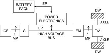
Figure 7.27 Series HEV schematic.
In this SHV, the ICE drives a generator (G) and has no direct mechanical connection to the drive axles. The vehicle is propelled by the electric motor (EM), which receives its input electrical power from a high-voltage bus. This bus, in turn, receives its power either from the engine-driven generator (for ICE propulsion) or from the battery pack (for EM propulsion), or from a combination of the two. In this figure, mechanical power is denoted MP and electrical power EP. The mechanical connection from the EM to the transaxle (T/A) provides propulsive power to the drive wheels (DWs). The term transaxle refers to the entire drive system from the EM to the drive wheels.
Figure 7.28 is a schematic of a hybrid vehicle type known as a parallel hybrid. The parallel hybrid of Figure 7.28 can operate with ICE alone by engaging both solenoid-operated clutches on either side of the EM but with no electrical power supplied to the EM. In this case, the MP supplied by the ICE directly drives the transaxle T/A, and the EM rotor spins essentially without any mechanical drag. This hybrid vehicle can also operate with the EM supplying propulsive power by switching off the ICE, disengaging clutch C1, engaging clutch C2, and providing electrical power to the EM from the high-voltage bus (HVB). Of course, if both ICE and EM are to produce propulsive power, then both clutches are engaged. Not shown in Figure 7.28 is a separate controller for the motor. Also not shown in this figure but discussed later in this section is the powertrain controller that optimizes performance and emissions for the overall vehicle and engages/disengages clutches as required.
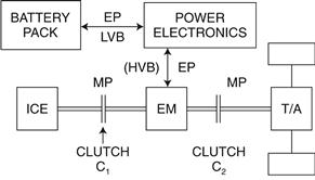
Figure 7.28 Parallel hybrid schematic.
The HEV of Figure 7.29 operates similarly to that of Figure 7.28 except that mechanical power from ICE and EM are combined in a mechanism denoted coupler. For the system of Figure 7.29 pure ICE propulsion involves engaging clutch C1, disengaging clutch C2, and providing no electrical power to the EM. Alternatively, pure EM propulsion involves disengaging clutch C1, switching off the ICE, engaging clutch C2, and providing electrical power to the EM via the high-voltage bus (HVB). Simultaneous ICE and EM propulsion involves running the ICE, providing electrical power to the EM, and engaging both clutches.
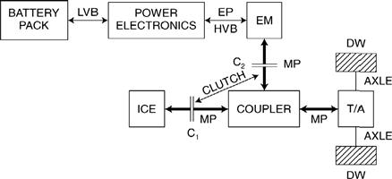
Figure 7.29 HEV with mechanical coupler.
In principle, any type of electric motor could be used to provide the electric propulsion in a hybrid vehicle. However, in practice, there are two main types in common use today: the brushless DC motor and the induction motor. Both are explained and modeled in Chapter 6. It should be recalled that the brushless DC motor incorporates a permanent magnet rotor normally with multiple poles. The stator has multiple windings that are excited by AC currents. Typically, the stator windings are arranged for three-phase operation.
However, the stored electric power in a hybrid vehicle is DC (from the battery pack). The frequency condition for this type of motor requires that the rotational frequency ωm be identical to the stator excitation frequency ωs since the rotor excitation is at ωr = 0.
Operation of the brushless DC motor in a hybrid vehicle during electric propulsion requires that an electric system convert the stored DC electric power to 3-phase AC power. This conversion is accomplished in a motor control system that creates an electric control signal at frequency ωs in addition to power switching circuits (normally implemented via high-power switching transistors). Ideally, the stator excitation should be three sinusoidal voltages of equal amplitude which in phasor notation are given by
 (62)
(62)
However, in practice, the excitation waveforms are not sinusoidal. Rather, they are more often of a form of square or trapezoidal waveform. Motor control requires correct phasing relative to the orientation of the rotor. Such phasing requires a noncontacting rotor position sensor (e.g., Hall effect; see Chapter 6).
In order to provide torque and power levels required for hybrid vehicle operation a brushless DC motor is made using powerful magnets having so-called rare earth elements. A typical magnet for a hybrid vehicle brushless DC motor is made of an alloy of iron, boron, and, the relatively expensive rare earth, element, neodynium.
A brushless DC motor can also function as an alternator. The motion of the rotor creates a time-varying flux linking the stator turns ФA, ФB, and ФC. This time-varying flux linkage, in turn, creates a voltage given by VAVBVC in each winding:

The zero phase corresponds to the rotor rotation angle for which ФA is a maximum.
These voltages can be converted to DC using a set of transformers (to achieve correct voltage levels) and rectifier circuits (see Chapter 3). The corresponding DC power can be supplied to the battery pack to increase its state of charge. In this way, the motor acting as a generator can provide braking torque to decelerate the vehicle and recover some of the vehicle kinetic energy that would otherwise be dissipated in brakes. Such generator action is known as regenerative braking.
Other electric motor types also have application in hybrid vehicle propulsion. In Chapter 6 the induction motor was explained. Induction motors of high torque/power output and high efficiency can be built without requiring rare earth magnetic material. A model for an induction motor was presented in Chapter 6 where it was shown that the frequency condition for average torque generation is automatically satisfied.
Induction motors for hybrid vehicle use are normally three-phase, meaning that three separate windings (one for each phase) are required for both stator and rotor. In Chapter 6 it was shown that the torque produced by the induction machine (with current excitation amplitude Is) is given by
 (63)
(63)
where ωs is the excitation frequency and ωm is the motor rotational frequency.
All parameters in this model for Te are defined in Chapter 6. It is also shown in Chapter 6 that the steady-state motor speed for a given excitation is the motor angular speed ωo at which the motor torque Te(ωo) balances the load torque TL:
![]() (64)
(64)
This point is illustrated for a hypothetical hybrid vehicle being propelled solely by an induction motor. The load torque at the motor output is proportional to the force FV required to move the vehicle at the commanded speed.
We consider first a hybrid vehicle moving along a steady speed on a straight, level road. There are two primary contributions to FV: tire rolling resistance Frr and aerodynamic drag D. The rolling resistance is essentially independent of vehicle speed but is proportional to vehicle weight and varies as a decreasing function of tire pressure. If we assume that all tires are equally inflated, then the total rolling resistance force is given by
![]()
where WV is the vehicle weight and μrr is the coefficient of rolling resistance of tires. The coefficient μrr is generally in the range 0.02 ≤ .μrr ≤ 0.04.
The aerodynamic drag D is given by
![]()
where ρ is the local air density (kg/m3 or slug/ft3), CD is the drag coefficient, Sref is the a reference area (m2 or ft2), and V is the vehicle speed (m/s or ft/s).
The reference area is an arbitrary choice that ultimately determines the value for CD. It is common practice to choose Sref as the vehicle projected area on a vertical plane normal to the vehicle plane of symmetry. The force necessary to move the vehicle along a straight, level road at a constant speed V is given by
![]()
The above expression for FV is valid for a level road. Whenever the vehicle encounters a nonzero slope (i.e., along a hill), this force includes a term that is proportional to the vehicle weight and the slope of the hill. For a vehicle traveling along a road with a slope (relative to horizontal) of angle θ, the total force FV is given by
![]() (66)
(66)
Thus, a road with nonzero slope can shift load torque on the motor (TL) up or down depending upon whether sign (θ) is + or θ, respectively.
In the hypothetical example, the induction motor drives the vehicle wheels through a transmission and differential such that ωm is proportional to V. The load torque at the motor output TV is proportional to the force FV:
![]() (67)
(67)
where gV is the gear ratio from motor to drive wheels and rT is the tire effective radius.
Figure 7.30 is a plot of normalized motor torque Tm and load torque TL (normalized to the maximum motor torque Tmax) vs. the ratio ωm/ωs where
![]()
![]()
where for a given excitation Tmax is defined as
![]()
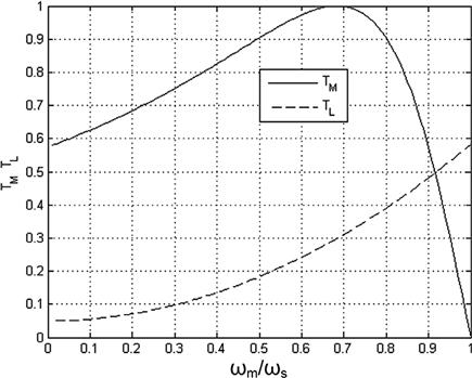
Figure 7.30 Normalized motor torque TM vs. normalized load torque TL.
The steady-state operating motor speed is at the intersection of these two curves (i.e., at ![]() ). A change in load torque (e.g., due to a nonzero road slope) causes the load curve to shift to a new motor operating point. The system is stable as long as
). A change in load torque (e.g., due to a nonzero road slope) causes the load curve to shift to a new motor operating point. The system is stable as long as
![]()
The efficiency of the induction motor is influenced, in part, by the steady-state operating point. In general, as long as the steady-state operating point (i.e., ωm = ωo) is in the negative slope region of Te(ωm) (and operation is stable), the motor produces torque that varies in proportion to slip s. However, motor efficiency varies inversely with slip.
The induction motor controller can regulate Te(ωm) via the excitation frequency (ωs) and current amplitude Is or motor voltage Vs. One hypothetical control strategy would vary the excitation and synchronous excitation frequency (ωs) to optimize the motor efficiency. However, there are many other factors that influence the overall vehicle efficiency including the choice of ICE and/or electric propulsion, battery status, vehicle-operating conditions and driving patterns (e.g., urban or highway), etc.
The current that provides the induction motor excitation Is is determined by the source voltage Vs and motor impedance. Normally, motor control is preferably done via regulation of Vs directly rather than via Is. We consider next the model for the motor torque based upon the excitation voltage Vs.
The stator current magnitude Is is related to the complex terminal voltage amplitude Vs. For sinusoidal excitation and using the parameter notation for induction motors from Chapter 6, the relationship between Vs and Is is given by
 (68)
(68)
This expression gives the voltage/current relationships for each phase. See Chapter 6 for the definitions of all parameters. Solving the above equation for Is and substituting it into the equation for motor torque yields
 (69)
(69)
The above equation provides a basis for motor torque control in hybrid vehicle applications.
For an induction motor at constant supply voltage amplitude Vs the slip s will vary until the motor torque is the same as load torque TL:
![]()
There is a family of curves of Te(s) for each excitation voltage that is similar in form to that given for current excitation (see Figure 7.30). Normal operation of an induction motor is in a region in which
![]()
and s is relatively small. In this region, the motor torque is given approximately by
 (70)
(70)
On the other hand, when slip is relatively large the torque can be shown to be given approximately by
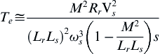 (71)
(71)
The above approximate expressions can be used to control motor torque for the two distinct regions of operation. In any event, the motor control can regulate torque by controlling excitation voltage as well as frequency ωs as explained later in this chapter.
For either series or parallel hybrid vehicle, dynamic braking is possible during vehicle deceleration, with the EM acting as a generator. The EM/generator supplies power to the high-voltage bus which is converted to the low-voltage bus (LVB) voltage level by the power electronics subsystem. In this deceleration circumstance, the energy that began as vehicle kinetic energy is recovered with the motor acting as a generator and is stored in the battery pack. This storage of energy occurs as an increase in the state of charge (SOC) of the battery pack. This process (regenerative braking) was discussed above with respect to the brushless DC motor, but applies equally well with an induction motor drive system.
In addition to the lead acid battery in common use today, there are new energy storage means including nickel–metal hydride (NiMH) and even special capacitors called ultra-caps. Each of these electrical energy storage technologies has advantages and disadvantages for hybrid vehicle application.
The battery pack has a maximum SOC that is fixed by its capacity. Dynamic braking is available as an energy recovery strategy as long as SOC is below its maximum value. Nevertheless, dynamic braking is an important part of hybrid vehicle fuel efficiency. It is the only way some of the energy supplied by the ICE and/or EM can be recovered when the vehicle is traveling along a road with a negative slope or is decelerating instead of being dissipated in the vehicle brakes.
For each battery type, there is a maximum rated stored charge qr which is determined by construction. The SOC for the battery is normally expressed by the instantaneous q expressed as a fraction of qr. A storage battery is, in effect, a type of nonlinear capacitor (with a nonlinear source resistance) in which the open circuit voltage Voc is a function of stored charge q:
![]()
The storage of the energy recovered during dynamic braking requires that the corresponding electrical energy be direct current and at a voltage compatible with the battery pack. Since most automotive systems apart from the motor operate at 12 V (nom), a common battery pack might consist of a connection of multiple 12-volt batteries.
Conversion of electrical power from one voltage level V1 to a second V2 is straightforward using a transformer as long as this power is alternating current. Figure 7.31 schematically illustrates transformer structure and the conversion of voltages from one level to another.

Figure 7.31 Transformer configuration.
A transformer consists of a core of magnetically permeable material (usually a ferromagnetic material) around which a pair of closely wrapped coils are formed. One coil (termed the primary) consists of N1 turns and the other (termed the secondary) consists of N2 turns. In a well-designed transformer essentially all of the magnetic flux in the core links all turns in both coils.
Assuming (arbitrarily) that AC electrical power comes from a source (e.g., an AC generator) at peak voltage V1, then the power flowing from the transformer secondary to a load will be at a peak voltage V2 where
![]()
Conversion of DC electrical power from one voltage to another can be accomplished using a transformer only if the DC power is first converted to AC and then converted back to DC as explained below. Figure 7.32a is a greatly simplified schematic of a DC-to-DC converter in which a transistor is used to convert an input DC signal to AC that is sent to a transformer for conversion to a different voltage.
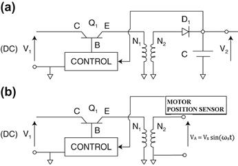
Figure 7.32 Voltage conversion circuit.
The control electronics supplies a pulsating signal to the base B of transistor Q1, alternately switching it on and off. When Q1 is on (i.e., conducting), voltage V1 is applied to the transformer primary (i.e., N1). When Q1 is off (i.e., nonconducting), transformer primary voltage is zero. In this case, the pulsating AC voltage that is alternately V1 and 0 applied to the primary results in an AC voltage in the secondary that is essentially N2/N1 times the primary voltage. This secondary voltage is converted to DC by rectification using diode D1 and filtering via capacitor C (see Chapter 3). The secondary voltage is fed back to the control electronics, which varies the relative ON and OFF times to maintain V2 at the desired level.
A variation of the circuit of Figure 7.32a appears in the power electronics module for conversion between the battery pack or from an ICE-driven generator and the hybrid vehicle motor driver. Regardless of the type of motor used, the generation of the voltages that provide the motor excitation (i.e., VA VB VC for a three-phase motor) can be accomplished using circuits of the configuration shown in Figure 7.32b. Although this figure depicts a single phase (i.e., VA), a separate driver transistor such as Q1 along with a transformer (of N1 primary and N2 secondary turns) is required for each phase. The control electronics internally computes the signals that control the phases (i.e., 0, 2π/3 and 4π/3) of the remaining three phases. This control is normally implemented in the powertrain control system. Of course, the specific details of the relevant power electronics depend on the hybrid vehicle manufacturer.
Powertrain control for a hybrid vehicle is achieved using a multimode digital control system. It is somewhat more complicated than the digital engine control system discussed earlier in this chapter in that it must control an IC engine as well as an EM motor. In addition, it must achieve the balance between ICE and EM power, and it must engage or disengage the solenoid-operated clutches (if present).
The inputs to this controller come from sensors that measure the following:
• power demand from driver (accelerator pedal),
• state of charge of battery pack,
The system outputs include control signals to
Depending upon the HEV configuration, there may be no direct mechanical link from the accelerator pedal to the throttle. Rather, the throttle position (as measured by a sensor) is set by the control system via an electrical signal sent to an actuator (motor) that moves the throttle in a system called drive-by-wire.
The control system itself is a digital controller using the inputs and outputs listed above and has the capability of controlling the hybrid powertrain in many different modes. These modes include starting from a standing stop, steady cruise, regenerative braking, recharging battery pack, and many others that are specific to a particular vehicle configuration.
In almost all circumstances, it is desirable for the IC engine to be off at all vehicle stops. Clearly, it is a waste of fuel and an unnecessary contribution to exhaust emissions for an IC engine to run in a stopped vehicle. Exceptions to this rule involve cold weather operations in which it is desirable or even necessary to have some limited engine operations with a stopped vehicle in order to maintain engine and catalytic converter at proper temperature. In addition, a low-battery SOC might call for ICE operation at certain vehicle stops in order to provide charge to the battery pack.
When starting from a standing start, normally the EM propulsion is used to accelerate the car to desired speed, assuming the battery has sufficient charge. If charge is low, then the controller can engage the clutch to the ICE such that the EM can begin acceleration and at the same time crank the ICE to start it. Then, depending on the time that the vehicle is in motion, the ICE can provide propulsive power and/or battery charge. Should the vehicle go to a steady cruise at low battery SOC for engine operation near its optimum, then the control strategy normally is to switch off the electric power to the EM and power the vehicle solely and recharge the battery pack with the ICE. In other cruise conditions, the controller can balance power between ICE and EM in a way that maximizes total fuel economy (subject to emission constraints).
For urban driving with frequent stops, the control strategy favors EM operation as long as SOC is sufficient. In this operating mode, regenerative braking may be used (in which energy is absorbed by vehicle deceleration), and the recovered energy appears as increased SOC.
The various operating modes and control strategies for an HEV depend on many factors, including vehicle weight; relative size and power capacity of ICE/EM; and exhaust emissions and fuel economy of the ICE (as installed in the particular vehicle). It is beyond the scope of this book to attempt to cover all possible operating modes for all HEV configurations. However, the above discussion has provided background within which specific HEV configurations’ operating modes and control strategies can be understood.
In addition to the HEV, there is also the pure electric vehicle (EV) that has no ICE for powering the vehicle. This vehicle incorporates many of the components of an HEV including an electric motor, a battery pack for storing electric energy, and an electronic controller that provides the motor excitation. As any EV is driven, the battery SOC decreases.
Control of the EM in an EV is accomplished in a way that is similar to that described above for EM motor control in an HEV. This control is done by regulating the excitation voltage or current as well as the excitation frequency (which must satisfy the frequency condition for any motor). At some point, the battery pack requires recharging. The power for this recharging comes from the electric power grid. It is worth remembering that although an EV has essentially zero vehicle-out emissions, the creation of the electric power to recharge the batteries is done at some electric utility. Depending on the type of power generation at the electric utility, there may be increased emissions from that plant to meet the power requirements to recharge EV battery packs except for nuclear electric power generators. In this sense, the EV is not always a pure zero-emission vehicle.
∗Dynamic Models for Torque Converter Equipped Vehicles, Allen Kotwicki, SAE paper # 820393, 1982.