
Chapter 10
Diagnostics and Occupant Protection
Chapter Outline
Electronic Control System Diagnostics
Model-Based Sensor Failure Detection
Model-Based Misfire Detection System
From the earliest days of the commercial sale of the automobile, it has been obvious that maintenance is required to keep automobiles operating properly. Of course, automobile dealerships have provided this service for years, as have independent repair shops and service stations. Until the early 1970s, however, a great deal of the routine maintenance and repair was done by car owners themselves, using inexpensive tools and equipment. However, the Clean Air Act affected not only the emissions produced by automobiles but also the complexity of the engine control systems and, as a result, the complexity of automobile maintenance and repair. Car owners can no longer, as a matter of course, do their own maintenance and repairs on certain automotive subsystems (particularly the engine). In fact, the traditional shop manual used for years by technicians for repairing cars is rapidly becoming obsolete and is being replaced by electronic technician aids.
As will be shown later in this chapter, the trend in automotive maintenance is for the automobile manufacturer to distribute all required documentation, including parts lists (with figures) as well as repair procedures in electronic format via a dedicated communication link (e.g. via satellite) or via CD supplied to the service technician. The repair information is then available to the technician at the repair site by use of a PC-like workstation.
Onboard digital systems can also store diagnostic information wherever a failure or partial failure occurs in a component or subsystem. The relevant information can then be stored in a memory (e.g. RAM) that retains the information even if the car ignition is switched off. Then, when the car is delivered to a repair station (e.g. at the dealer), the technician can retrieve the diagnostic information electronically.
The change from traditional fluidic/pneumatic engine controls to microprocessor-based electronic engine controls was a direct result of the need to control automobile emissions, and has been chronicled throughout this book. However, little has been said thus far about the diagnostic problems involved in electronically controlled engines. This type of diagnostics requires a fundamentally different approach than that for traditionally controlled engines because it requires more sophisticated equipment than was required for diagnostics in pre-emission control automobiles. In fact, the best diagnostic methods use special-purpose computers that are themselves microprocessor based.
Electronic Control System Diagnostics
Each microprocessor-based electronic subsystem has the capability of performing some limited self-diagnosis. A subsystem can, for example, detect a loss of signal from a sensor or detect an open circuit in an actuator circuit as well as other failures. As long as the subsystem computer is still functioning, it can store fault codes for detected failures. Such diagnosis within a given subsystem is known as onboard diagnosis.
Some limited self-diagnostics have been available in power train control from the earliest days of microprocessor-based control systems. However, the Environmental Protection Agency (EPA) has developed regulations mandating a relatively high level of diagnosis for components and subsystems that can adversely effect exhaust emissions when failed or in degraded performance. These regulations are known as “On-Board Diagnostics II” (OBD II). They require that the vehicle has within its electronic control/instrumentation systems the capability of essentially continuously monitoring the performance of the vehicle emission control systems. The details of this regulation and specific implementation schemes are discussed later in this chapter.
Whenever a fault in a component or system is detected, a code, specific to the failure/degraded performance known as a “Fault-code,” is stored in memory. Various techniques for detecting such failures are discussed later in this chapter. If the fault has the potential to degrade the emission control system beyond allowable limits, OBD II requires that the driver be alerted via a “check engine” message on the instrument panel.
However, a higher level of diagnosis than the onboard diagnosis is typically done with an external computer-based system that is available in a service shop. Data stored in memory in an onboard subsystem are useful for completing diagnosis of any problem with the associated subsystem. Such diagnosis is known as off-board diagnosis and is usually conducted with a special-purpose computer.
In order for fault code data to be available to the off-board diagnosis computer, a communication link is required between the off-board equipment and the particular subsystem on board the vehicle. Such a communication system is typically in the form of a serial digital data link. A serial data link transmits digital data in a binary time sequence along a pair of wires. Before discussing the details of onboard and off-board diagnosis, it is perhaps worthwhile to discuss briefly automotive digital communications.
It was shown in the previous chapter that the various electronic subsystems (ECUs) in a contemporary vehicle are connected together via the CAN network. For example, in Figure 9.34 one of the connections to the CAN bus is a data link (denoted DLC) that is a portal from the vehicle to the off-board diagnosis system. A connection is made to this diagnostic system when the vehicle is in an authorized repair facility (e.g. car dealer) for maintenance/repair.
Figure 10.1 depicts a representative connection of an off-board connection of a so-called diagnostic scan tool to an automotive DLC. The diagnostic scan tool depicted in Figure 10.1 is portable and can be carried in the vehicle when it is being test driven by a maintenance technician as discussed later in this chapter.

Figure 10.1 Illustration of diagnostic scan tool connection to vehicle.
The scanner has access to address and data buses of the subsystem containing the memory in which the relevant fault codes are stored. The scanner then sends addresses to the memory locations where the fault codes are stored and retrieves any fault code in each memory location associated with fault code storage. The scanner also includes a display device where it displays the fault code. Some diagnostic systems include storing the clock time of the occurrence of the fault. Such a system is useful for diagnosing intermittent faults (i.e. those that come and go randomly and are challenging for the technician to find). In addition to the portable scan diagnostic tool (PSDT), there is a service bay diagnostic tool (SBDT) which is often on a movable cart but is not small enough to be carried on board for test drivers.
Service Bay Diagnostic Tool
An alternative to the onboard diagnostics is available in the form of a service bay diagnostic system. This system uses a computer that has a greater diagnostic capability than the vehicle-based system because its computer is typically much larger and has only a single task to perform—that of diagnosing problems in vehicle electronic systems.
Service bay diagnostic systems are computer-based instruments that are capable of reading fault codes that are stored by the onboard diagnostic systems (e.g. via the DLC described in Chapter 9). In addition, they have electronic versions of the equivalent of shop manuals as well as recommended procedures for diagnosing specific problems from the stored fault codes as well as information and problem descriptions from the driver.
In certain circumstances, fault codes, by themselves, are insufficient to fully diagnose a given problem. In the cases, the off-board diagnostic system can present a sequence of steps that require action by the service technician which, when followed, can complete the diagnosis of a problem. Of course, it should be emphasized that fault codes are only applicable to those automotive systems/subsystems that have electrical or electronic components. Other subsystem/components require the knowledge and experience of the service technician to perform diagnosis/repair. For example, a failed or partially failed wheel bearing is not a failure that will have a stored fault code. The diagnosis and repair of problems in automobiles will always require competent, knowledgeable, trained technicians.
On the other hand, the electronic content in contemporary vehicles continues to increase with each new vehicle configuration/model. Thus, it is clear that electronic diagnostic methods will continue to proliferate.
In addition to storing and displaying shop manual data and procedures, a computer-based service bay diagnostic system has the theoretical capability to automate the diagnostic process itself. In achieving this objective, the technicians’ terminal has the capability to incorporate what is commonly called an expert system that is explained in detail later in this chapter.
Onboard Diagnostics
Onboard diagnostics are dictated largely by the need for each automobile to meet the requirements of OBD II regulations. As stated above, any component/subsystem having the potential to adversely affect exhaust emissions must be evaluated for its performance. In addition, however, on a power train systems level, the onboard diagnostics must be capable of detecting engine misfire. A misfire is any failure of any cylinder (during an engine cycle) to experience normal combustion. It can include e.g. a complete misfire in which ignition fails to cause combustion to occur. Partial combustion in which only a portion of the fuel/air mixture is combusted also can constitute a misfire by OBD II standards. A misfire can degrade the performance of the catalytic converter since the exhaust gas constituents and concentrations are outside the limits in which it is intended to function.
Any engine can experience an occasional, spurious misfire (or partial misfire). However, when the severity and frequency of occurrence exceeds certain tolerance limits the catalytic converter performance is degraded and exhaust emissions can exceed the EPA mandated limits. For such an occurrence, the warning message must be displayed and the owner should seek repairs for the vehicle. The format for this warning message varies with vehicle model, but it is often an illuminated “check engine” display. For convenience in the present chapter, this warning message is termed “fault indication lamp” or FIL since it is actually illuminated due to a component/system fault. An exemplary method of detecting misfires is described in detail later in this chapter.
On a component level, there are many individual components which can adversely affect exhaust emissions during periods of degraded performance. For example, the heated exhaust gas oxygen concentration sensor (HEGO; see Chapter 6) which is used for closed-loop fuel control can experience a failure or partial failure. For a warmed engine running with fuel control in closed-loop mode, the voltage waveform of the HEGO sensor will have certain patterns when the sensor is operating normally. This voltage should be cycling between its normal high voltage level (about 1 V) and its low voltage level (about 0.1 V). Moreover, the mean value of the sensor voltage will lie within a relatively narrow band that is approximately midway between the high and low voltage levels.
Any deviation in the HEGO sensor voltage waveform is an indication of a potential HEGO sensor failure or degraded performance. However, there are other potential causes of waveform parameters (HEGO sensor) outside expected limits. For example, the fuel control system could have experienced a failure and could be unintentionally fueling the engine too rich or too lean. In addition, one or more fuel injectors could have failed resulting in excessively rich or lean mixture.
The OBD II requirement at this point is to illuminate the FIL warning and set the appropriate fault codes. These might include separate codes corresponding to the conditions: (1) HEGO sensor voltage a steady high or (2) a steady low, (3) HEGO sensor voltage failure to cycle; (4) mean HEGO sensor voltage above limits or (5) below limits.
When the vehicle is brought to the service facility, the service technician will normally connect the appropriate off-board system to the DLC (see Figure 9.34) and transfer all fault codes from the onboard memory to the scan tool. With all fault codes present the service technician can follow a set of procedures to diagnose the failures.
Another component that can fail affecting exhaust emissions is a fuel injector. Not all fuel injector failures are detectable with onboard diagnostics. However, the power train control system can monitor fuel injector current and terminal voltage. Measurement of these quantities can detect an open or short circuit in the fuel injector solenoid coil. Of course, should either condition be detected OBD II requires the driver alert message as well as storage of the appropriate code and identification of the affected cylinder.
Still another important component requiring monitoring is the catalytic converter. As stated earlier in this book, there is no cost-effective way of measuring the regulated exhaust gas concentrations on board the vehicle. On the other hand, it is possible to obtain some assessment of the catalytic converter conversion efficiency by placing a second HEGO sensor in its output side. The primary HEGO sensor for fuel control is located upstream of the catalytic converter. Recall from Chapter 7 that in closed-loop mode the fuel control continuously cycles from rich to lean of stoichiometry and from lean to rich. During periods of relatively rich mixture the exhaust gas oxygen concentration is low. This exhaust gas enters the catalytic converter with the low O2 concentration where the converter acts as an oxidizer. The reverse is true for a relatively lean mixture. A comparison of the primary and secondary HEGO sensor voltages can serve as an indication of relative converter efficiency.
Model-Based Sensor Failure Detection
The performance of certain sensors can be evaluated via model-based calculation from measurements of other sensors. For example, the MAF is an important sensor for setting fuel injector base pulse duration (see Chapter 7). A calibration change in the MAF sensor can lead to misfueling (relative to stoichiometry) particularly in open-loop mode of fuel control. It is important to maintain proper fuel/air mixture regardless of the controller mode of operation.
An independent check on MAF calibration is possible (theoretically) for any engine that also has an MAP sensor and an intake air temperature sensor. Assuming that these sensors are functioning correctly the mass flow rate ![]() into the intake system is given by:
into the intake system is given by:
![]() (1)
(1)
where ![]()
δi = intake air density.
Using tables of volumetric efficiency (ηV) for the engine as a function of throttle angle and RPM, the volume flow rate ![]() is given by:
is given by:
![]() (2)
(2)
where De = engine displacement
n = R/60
R = RPM
θt = throttle angle.
The intake air density is given by
![]() (3)
(3)
where δ0 = sea-level standard day air density
p0 = sea-level standard day air pressure
T0 = sea-level standard day air temperature
pi = intake manifold air pressure
Ti = intake manifold air temperature.
In principle, the MAF sensor calibration can be evaluated by comparing the measured value of ![]() from it with the calculated value from temperature and pressure measurements. Unfortunately, the cost of adding extra sensors makes it unattractive to an automobile manufacturer to implement such a method unless these sensors were already in place for other control applications. Nevertheless, this hypothetical example illustrates the potential for cross-checking the performance of various sensors.
from it with the calculated value from temperature and pressure measurements. Unfortunately, the cost of adding extra sensors makes it unattractive to an automobile manufacturer to implement such a method unless these sensors were already in place for other control applications. Nevertheless, this hypothetical example illustrates the potential for cross-checking the performance of various sensors.
It has been shown (e.g. see Chapter 7) that power train control uses numerous angular speed sensors. As shown in Chapter 6 many of these use a magnetic or optical sensor in conjunction with a disk having multiple lugs. Many failure modes are possible with such sensors. For example, a magnetic speed sensor incorporating a permanent magnet and a coil can experience shorting of a portion of the coil turns. This type of failure leads to a lower than normal output voltage at any given speed. Although speed measurement from such a sensor is based upon the frequency of counted pulses, the failure can occur whenever the voltage amplitude falls below the level at which the signal processing can detect the presence of some (or all) of the pulses produced within one revolution. In addition it is possible for one of the lugs to come off the disk (e.g. due to manufacturing defect). In either type of failure the signal processing will compute an incorrect angular speed for the sensor.
One method for detecting missing pulses uses the controller clock to record the time of occurrence tk(k = 1, 2, … K) of each of the pulses in the incoming sequence during any given engine cycle where K is the number of lugs on the disk. The controller can also obtain the differential time between successive pulses
![]()
If a sensor failure of the types described above has occurred then there will be at least one differential time which is significantly different from the others in a full sequence during an engine cycle. The measurements of angular speed for this particular time differential is termed an outlyer. Several standard algorithms exist for detecting and removing these erroneous measurements from the data collected during each cycle of operations as well as setting a fault code.
Various temperature (e.g. coolant temperature) sensors are used in power train control whose accuracy affects emission control. The very wide range of temperatures over which a vehicle operates essentially precludes a practical and reliable means of checking the calibration accuracy. On the other hand, open and short circuit conditions can be detected by monitoring sensor terminal voltages. However, depending upon the design, it may be possible to establish limits on the possible range of indicated temperatures. Any reading outside this range can be considered a detected fault.
In addition to those sensors that must be monitored for OBD II requirements, there are sensors that are important for safe reliable vehicle operation. For example, an oil pressure measurement is important to assure that proper lubrication is present for all engine rotating parts. Such sensors can be monitored with respect to open/short circuit conditions.
In addition, the proper operation of electrical system is important. The charging of the battery via the alternator can be monitored by both the terminal voltage and the current flow. In particular, an alternator voltage level that is too low or too high for engine operating conditions is an indication of an alternator problem.
As will be demonstrated below, the diagnostic capability provided in any modern microprocessor-based electronic control system (although somewhat limited) can provide valuable assistance to the service technician. These diagnostic functions are performed by the microprocessor under the control of stored programs, and are normally performed when the microprocessor is not fully committed to performing normal control calculations. While it is beyond the scope of this book to review the actual software involved in such diagnostic operations, the diagnostic procedures that are followed and explanations of onboard diagnostic functions can be reviewed, by example.
During the normal operation of the car, there are periods during which the performance of various electrical and electronic components is monitored via the vehicle instrumentation system (see Chapter 9). Whenever a fault is detected, the data are stored in memory using a specific fault code. At the same time, the controller generates or activates an FIL warning lamp (or similar display) on the instrument panel indicating that service is required provided the fault affects the emission control system or affects safety.
The onboard diagnostic functions have one major limitation—they cannot detect intermittent failures reliably. For the system to detect and isolate a failure, the failure must be nonreversible and persistent. In an onboard diagnostic system, if the electronic control module stores trouble codes that are automatically cleared by the microprocessor after a set number of engine cycles have occurred without a fault reappearing, then intermittent failure detection is precluded. However, it is possible in certain vehicles for the system to be put into a fault-recording mode. Many times such a fault-recording mode can identify intermittent failures.
Diagnostic Fault Codes
The Society of Automotive Engineers (SAE) has developed a set of recommended practices that provides a standard set of diagnostic fault codes for those component/system faults that are common to all vehicle models. By standardizing fault codes, a qualified independent service technician can diagnose certain problems on any vehicle using a universal scan tool. Each individual car manufacturer defines its own fault codes for any component or system that is not encompassed by the standard set.
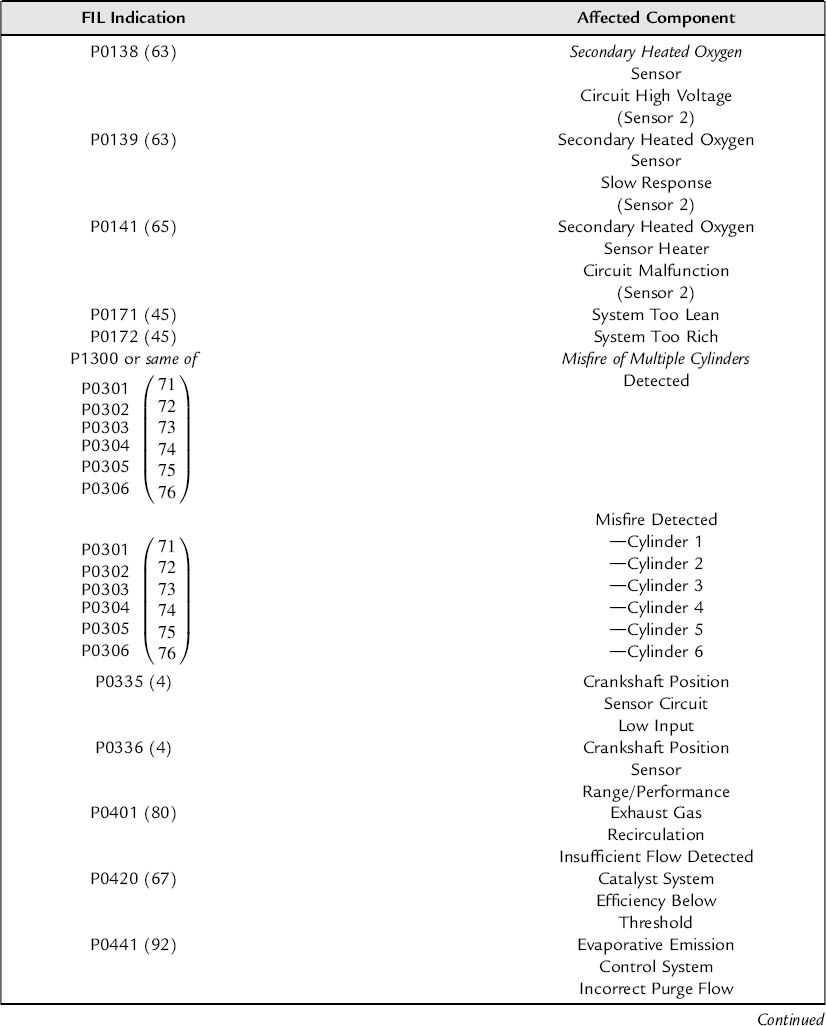
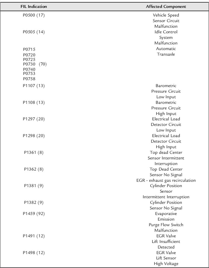
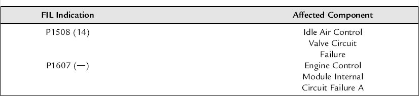
The SAE-defined code has the format P0xxx. A partial list is given in Table 10.1 as an example of a subset of fault codes. Manufacturer-specific codes can have a format P1xxx as illustrated in Table 10.1.
Table 10.1 Fault code sample.

The procedure for diagnosing one or more problems during vehicle repair/maintenance begins with the service technician connecting the off-board diagnostic scan tool to the DLC. With the ignition switch on and this tool connected, data associated with any or all faults are automatically transferred to the diagnostic tool. In addition to the individual fault codes that were stored, additional data indicating the engine and associated components/systems operating conditions may also be transferred (depending on the vehicle model and manufacturer).
In most cases, the most advanced diagnostic tools are computer based having relatively large databases related to diagnostic and repair procedures. Commonly, these procedures are presented to the service technician in the form of a flowchart (not unlike a flowchart for a computer algorithm). The flowchart appears on the diagnostic tool visual monitor (e.g. computer display) in a graphical/pictorial form. Although the procedures to be followed in the flowchart depend on the particular fault, it is possible to illustrate the procedures with a representative example. The example taken here considers a failure in the primary HEGO. Refer to Chapter 7 for a review of the role played by this important sensor in closed-loop fuel control.
Once the vehicle has been taken (possibly driven) to an authorized repair facility, the diagnosis begins with the service technician connecting the diagnostic (scan) tool to the DLC. If the onboard diagnostic subsystem has detected an HEGO sensor low voltage fault, it will store the fault code P0131 in memory (see Table 10.1). When properly connected, either of the scan tools (i.e. PSDT or SBDT) will display this code to the service technician. For our example situation, it is presumed that the service bay scan tool has the relevant diagnostic flowchart stored internal to its computer and will display (either automatically or at the command of the technician) a flowchart such as is depicted in Figure 10.2.
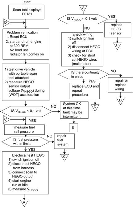
Figure 10.2 Flowchart for diagnosing fault in primary HEGO.
The first step in the procedure of this flowchart involves verification that a fault has actually occurred and persists. This verification is accomplished during a test drive with a fully warmed vehicle that is conducted by the service technician with the PSDT connected and configured to measure and display the primary HEGO sensor terminal voltage (VHEGO). If this voltage does not satisfy the condition (VHEGO ≤ 0.1 V), the system is deemed to be functioning properly at the time of the test drive and the FIL is considered to be intermittent. For this test drive outcome, a separate path (denoted B in Figure 10.2) is to be followed. This path includes the recommendation that the service technician examine the wiring associated with the HEGO sensor to check for broken or loose wires or connectors. If no wiring problem is found and the vehicle has experienced other such FIL warnings, the instructions may be to install special recording equipment in the vehicle and either return it to service or repeat the test drive.
On the other hand, if VHEGO ≤ 0.1 V, the flow path directs the service technician to measure fuel pressure. If this pressure is outside limits specified in the service manual, it must be repaired. After repairs are completed, Step C involves returning to the flowchart at the point indicated.
If the fuel pressure is within limits, the service technician is directed to electrical tests of the HEGO. With the engine switched off, the HEGO is disconnected from the wiring harness. A diagnostic scan tool is connected via a set of leads with clip-on ends to the sensor terminals of the HEGO (note: for a HEGO, there is also a pair of connectors for the heating element; see Chapter 6). The engine is then started and allowed to idle. The HEGO voltage is measured by the scan tool. At this point in the flowchart, there is a break from point A to the continuous point A at the top right of the flowchart.
If the condition VHEGO ≤ 0.1 V is met, it is the HEGO sensor itself that has failed and it is replaced. To confirm that the problem has been resolved, the technician returns to point D in the procedure. Assuming that the problem is resolved, the procedure will end at point B where it will become concluded that the problem is fixed. If this condition is not met, the sensor is functioning and the problem of low HEGO sensor voltage may be in the wiring harness.
The next step in the flowchart involves testing the wiring harness from the HEGO to the engine control unit (ECU). The HEGO sensor wiring harness is removed from the ECU and a wire continuity test is performed using either the scan tool or any available multimeter. If there is either intermittent or no continuity in the sensor wires from the ECU to the sensor end and if there are short circuits either between the two sensor leads or from either to ground, the harness is faulty and must be repaired (if possible) or replaced. Again the procedure will be repeated at D and if the problem is resolved, the procedure will end in step B with a conclusion that the system is repaired.
If there is continuity, the problem must be in the ECU itself. The service technician is directed to replace the ECU with a known good one. If the problem with low HEGO sensor voltage disappears, a permanent replacement ECU is installed. At this point, there is a return to point D and if the problem has been resolved, the exit at step B is taken.
If, after the vehicle is returned to service, the FIL is illuminated and the scan tool detects fault P0131 again, the problem is an intermittent fault. Among the possible options is the choice of installing a recording device that can, over a period of time, collect data to identify that an intermittent fault has occurred. It is also possible to replace the HEGO sensor and its wiring harness and continue road testing.
Another example procedure will be illustrated here by following the steps necessary to respond to the specific fault code P0133, which indicates that the HEGO sensor has slow response. Recall from the discussion in Chapter 6 that the HEGO sensor switches between approximately 0.1 and 1 V as the mixture switches between the extreme conditions of lean and rich. Recall also that this voltage swing requires that the HEGO sensor must be at a temperature above 200 °C. Fault code P0133 means that the HEGO sensor may not swing above or below its cold voltage of approximately 0.5 V, and that the electronic control system will not go into closed-loop operation (see Chapters 5 and 7) or that the transitions are too slow for closed-loop control to function. Possible causes for fault code P0133 include the following:
• HEGO sensor is not functioning correctly.
• The connections or leads are defective.
• The control unit is not processing the HEGO sensor signal.
Further investigation was required to attempt to isolate the specific problem.
To check the operation of the HEGO sensor, the average value of its output voltage is measured using the scan tool (or a multi meter). The desired voltage is displayed on the scan tool.
Using this voltage, the service technician follows a procedure outlined in Figures 10.3 and 10.4. If the voltage is less than 0.37 V or greater than 0.57 V, the service technician is asked to investigate the wiring harness for defects.

Figure 10.3 Flowchart for diagnosis of HEGO sensor output voltage problems.
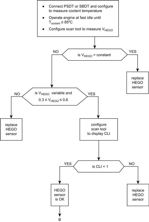
Figure 10.4 Flowchart for HEGO sensor proper switching sensor test.
If the HEGO sensor voltage is between 0.37 and 0.57 V, tests are performed to determine whether the HEGO sensor or the control unit is faulty. The service technician must jumper the HEGO sensor leads together at the input to the control unit, simulating a sensor short circuit, and must read the sensor voltage value using the PSDT (or a suitable multi meter). If this voltage is less than 0.05 V, the control unit is functioning correctly and the HEGO sensor must be investigated for defects. If the indicated sensor voltage is greater than 0.05 V, the control unit is faulty and should be replaced.
A further test of the proper HEGO sensor dynamic (switching) operation as part of the engine control is illustrated in the flowchart of Figure 10.4. In this diagnostic procedure, the goal is to ascertain whether the HEGO sensor operation results in closed-loop mode of engine control. As explained in Chapter 7, the engine must be sufficiently warmed before closed-loop operation is activated. The first step in the flowchart is to run the engine and monitor coolant temperature. Once this temperature exceeds a given threshold level, the HEGO sensor should be operating properly even if the heater has failed. The technician is directed to run the engine at fast idle and monitor HEGO sensor voltage. Under these conditions, the sensor should be switching. If the voltage is constant, the sensor has failed and must be replaced.
If the sensor voltage is variable, it must switch from less than 0.3 V to more than 0.6 V. If it does not, it must be replaced. If it does meet this condition, the service technician is directed to determine if closed-loop mode is activated or not. The PSDT tool is configured to read a binary-valued parameter that is termed “closed-loop indicator” (CLI). If CLI = 0, the HEGO sensor switching is insufficient to cause closed-loop operation to occur and the sensor is replaced. If CLI = 1, the sensor is OK and this diagnostic procedure is complete. It should be noted that the ECU could also have failed, but diagnosis of this problem would follow a different flowchart.
In addition to measurement of HEGO sensor, the scan tool can be used by a service technician to measure other variables or parameters as suggested above. We consider, for example, the throttle position sensor which provides an important input to the electronic engine control as explained in Chapters 5, 6 and 7. The onboard diagnostic can detect out-of-limits values for this sensor and display fault codes, e.g. P0122 for voltage below a lower limit or P0123 for voltage above a high limit. However, other throttle position sensor faults are possible that are not detected by the exemplary onboard diagnostic system. A change in calibration of this sensor will normally result in an incorrect computation of fuel injector base pulse duration (see Chapter 7). Such a calibration failure could result from a change in the supply voltage to the sensor. Even though no fault code is set for such a failure (in this hypothetical example), a service technician with sufficient experience and knowledge may suspect such a failure if the vehicle driver reports an apparent reduction in performance under certain driving conditions. The technician can configure the scan tool to measure the throttle position sensor voltage. Then, with the ignition switch in the on position but with the engine not running, the service technician can measure the voltage as the throttle is depressed. Although it is theoretically possible to independently measure throttle angular position θt and to obtain a plot of sensor voltage Vt(θt), normally it is sufficient for diagnostic purposes to qualitatively examine the voltage as the throttle is changed. This sensor voltage should change smoothly and roughly linearly with θt. Similar measurements can be made on other sensors which might have developed partial failures (e.g. calibration shift) that are not sufficient to be detected by the onboard diagnostic system.
In addition to parameter and variable measurements, the diagnosis of problems with various switches is often desirable or even necessary. Various examples of the important function of certain switches have been explained in previous chapters. For example, in a cruise control system, the brake pedal switch has the critical safety-related function of disconnecting the throttle actuator from the throttle linkage in a cruise control system (see Chapter 8) when the driver applies the brakes. The onboard diagnostic system cannot detect a failure in this switch unless there is an independent means of sensing that brakes are applied (e.g. via a brake pressure sensor). Owing to this potentially inherent limitation of the onboard diagnostic system, it is desirable to perform a sequence of switch tests during a routine vehicle servicing procedure. The evaluation of various switches can be implemented automatically via the diagnostic tool with the involvement of the service technician. Such an automatic switch test procedure was implemented in at least one production vehicle.
We illustrate this switch test procedure with the above exemplary system in which the scan tool is configured to display two-digit diagnostic codes. The two-digit codes and associated circuit are presented in Figure 10.5. In this figure, the relevant diagnostic codes displayed on the scan tool are represented by digits AA.

Figure 10.5 Switch test sequence.
For this example, the switch tests involve diagnostic codes 71-80 and provide checks on the switches indicated in Figure 10.5.
To begin the switch tests, the service technician must depress and release the brake pedal. If there is no brake switch failure, then the code advances to 71. If the display does not advance, then the control unit is not processing the brake switch signal and further diagnosis is required. For such a failure, the service technician locates the specific flowchart (such as seen in Figure 10.6) for diagnosis of the particular switch failure and follows the procedure outlined. The detailed tests performed by the service technician are continuity checks that are performed with the PSDT or a multimeter. Figure 10.7 depicts the cruise control brake circuit diagram.
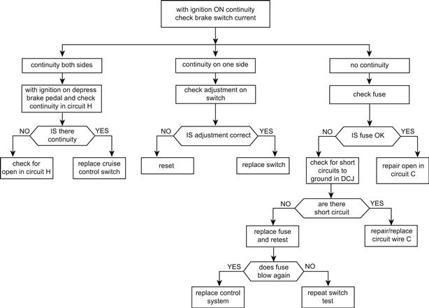
Figure 10.6 Cruise control brake circuit.

Figure 10.7 Cruise control brake circuit.
Whenever any switch test fails, a diagnostic flowchart is called up by the service technician, and its steps are followed in the sequence displayed on the scan tool. Similar procedures are followed for each switch test in the sequence. This procedure sequence is as follows:
(1) With code 71 displayed, depress and release brake pedal for normal operation, the display advances.
(2) With code 72 displayed, depress the throttle from idle position to wide-open position. The control unit tests the throttle switch, and advances the display to code 73 for normal operation.
(3) With code 73 displayed, the transmission selector is moved to drive and then neutral. This operation tests the drive switch, and the display advances to code 74 for normal operation.
(4) With code 74 displayed, the transmission selector is moved to reverse and then to park. This tests the reverse switch operation, and the display advances to code 75 for normal operation.
(5) With 75 displayed, the cruise control is switched from off to on and back to off, testing the cruise control switch. For normal operation, the display advances to 76.
(6) With code 76 displayed and the cruise control switch on, depress and release the set/coast button. If the button (switch) is operating normally, the display advances to 77.
(7) With 77 displayed and with the cruise control instrument on, depress and release the resume/acceleration switch. If the switch is operating normally, the display advances to 78.
(8) With 78 displayed, depress and release the instant/average button on the trip information computer (TIC). If the button is working normally, the code advances to 79.
(9) With 79 displayed, depress and release the reset button on the TIC panel. If the reset button is working normally, the code will advance to 80.
(10) With 80 displayed, depress and release the rear defogger button on the climate control head. If the defogger switch is working normally, the code advances to 70, thereby completing the switch tests.
This exemplary diagnostic tool can also be used to display certain engine parameters with the engine running (either in the service bay or on a road test). The scan tool gives the measurement as well as the normal range for the parameter.
Figure 10.8 shows the parameter values in sequence for an exemplary vehicle. Parameter 01 is the angular deflection of the throttle in degrees from idle position.
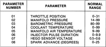
Figure 10.8 Chart of exemplary engine parameters with normal ranges.
Parameter 02 is the manifold absolute pressure in kilopascals. The range for this parameter is 14-99, with 14 representing about the maximum manifold vacuum. Parameter 03 is the absolute atmospheric pressure in kPa. Normal atmospheric pressure is roughly 90-100 kPa at sea level. Parameter 04 is the coolant temperature and Parameter 05 is the intake manifold temperature.
Parameter 06 is the duration of the fuel injector pulse in milliseconds. Refer to Chapters 5, 6, and 7 for an explanation of the injector pulse widths and the influence of these pulse widths on fuel mixture.
Parameter 07 is the average value for the HEGO sensor output voltage. Reference was made earlier in this chapter to the diagnostic use of this parameter. Recall that the HEGO sensor switches between about 0.1 and 1 V as the mixture oscillates between lean and rich. The displayed value is the time average for this voltage, which varies with the duty cycle of the mixture.
Parameter 08 is the spark advance in degrees before TDC. This value should agree with that obtained using a SBDT configured in the engine analyzer mode. Although it is not shown in Figure 10.8, parameter 09 is the number of ignition cycles that have occurred since a trouble code was set in memory. If 20 such cycles have occurred without a fault, this counter is set to zero and all trouble codes are cleared.
Parameter 10 (not shown in Figure 10.8) is a logical (binary) variable that indicates whether the engine control system is operating in open or closed loop (i.e. the CLI). A value of 1 corresponds to closed loop, which means that data from the HEGO sensor are fed back to the controller to be used in setting injector pulse duration. Zero for this variable indicates open-loop operation, as explained in Chapters 6 and 7. Parameter 11 is the battery voltage.
Onboard Diagnosis (OBD II)
Onboard diagnosis has also been mandated by government regulation, particularly if a vehicle failure could damage emission control systems. The relatively severe requirement for onboard diagnosis is known as OBD II. This requirement is intended to ensure that the emission control system is functioning as intended.
Automotive emission control systems, which have been discussed in Chapters 5 and 7, consist of fuel and ignition control for the three-way catalytic converter, as well as controls for EGR, secondary air injection, and evaporative emission. The OBD II regulations require real-time monitoring of the performance of the emission control system components. For example, the performance of the catalytic converter must be monitored using a temperature sensor for measuring converter temperature and a pair of HEGO sensors (one before and one after the converter).
Another requirement for OBD II is a misfire detection system. It is known that under misfiring conditions (failure of the mixture to ignite), exhaust emissions increase. In severe cases, the catalytic converter itself can be irreversibly damaged.
The only cost-effective means of meeting OBD II requirements involves electronic instrumentation. Owing to intellectual property issues, it is not feasible to present an actual misfire detection system used by any particular automotive manufacturer. Rather, we present a hypothetical misfire detection system that is mathematical model based and which has been tested under laboratory conditions as well as in actual road tests.
Model-Based Misfire Detection System
A model-based method of detecting engine misfires requires a dynamic model for the power train of sufficient detail and accuracy to be able to represent the relationship between the instantaneous torque fluctuations and the corresponding fluctuations in crankshaft instantaneous angular speed ωe(t). It is shown later in this section that measurements of ωe(t) can be used as the basis for misfire detection in accordance with the following model. The instantaneous net torque Tn applied at the flywheel consists of the algebraic sum:
![]() (4)
(4)
where θe(t) = crankshaft instantaneous angular position
Ti[θe(t)] = indicated torque
TR[θe(t)] = torque due to inertial forces of reciprocating components
TFp[θe(t)] = friction and pumping loss torque
Tl[θe(t)] = load torque from transmission.
The indicated torque is the torque that is applied to the crankshaft due to cylinder pressure during combustion acting on the piston area (Ap) through the instantaneous lever arm ![]() (θe) of the connecting rod crankshaft throw structure (see Chapter 5). The friction component of TFp is due to the sliding friction of all moving surfaces and the pumping component of TFp is the torque required to pump the fuel air mixture into each cylinder and pump the exhaust gases out of the engine through the exhaust system.
(θe) of the connecting rod crankshaft throw structure (see Chapter 5). The friction component of TFp is due to the sliding friction of all moving surfaces and the pumping component of TFp is the torque required to pump the fuel air mixture into each cylinder and pump the exhaust gases out of the engine through the exhaust system.
The reciprocating torque is the torque applied to the crankshaft due to the inertial forces associated with the reciprocating motion of the piston/connecting rod/crankshaft throw. This torque amplitude increases quadratically with RPM but can be computed with great accuracy for any given engine configuration from the known geometry and component masses.
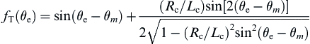
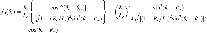
For the purposes of illustrating the present concept for misfire detection a number of simplifying assumptions are made. There is negligible loss of model robustness by assuming that the crankshaft is infinitely stiff and experiences insignificant torsional motion in response to the torque fluctuations. It is also adequate for the present purposes to assume that the connecting rod is sufficiently long relative to the crankshaft throw (Rc) and that the piston pin offset is negligible such that the indicated torque due to the power stroke of the mth cylinder is given by:
![]() (5)
(5)

and where Lc = connecting rod length
Rc = crankshaft throw
pc = cylinder pressure
po = atmospheric pressure
where θm = θe at TDC for cylinder m.
The origin for θe is taken as the crankshaft angle for the number 1 cylinder at TDC for compression/combustion strokes. The indicated torque is the sum of the indicated torque for all M cylinders of an M cylinder engine

The reciprocating torque associated with the mth cylinder are given by:
![]() (6)
(6)
![]()
 (7)
(7)
where: Meq = sum of the mass of the piston, wrist pin and 1/3 of the connecting rod.
The combined reciprocating torque TR is given by:
 (8)
(8)
For the purposes of modeling the engine for misfire detection, it is possible to approximate TFp(θe) with a linearized model as given below:
![]()
where Re = linearized friction coefficient.
The net torque applied to the crankshaft is the sum of the components:
![]() (9)
(9)
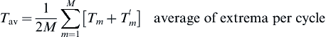
The present method of misfire detection in an engine is based upon a metric which represents the nonuniformity in torque generation (i.e. in δTk). If every cylinder produced exactly the same torque during a given engine cycle, the fluctuations in δTk would have exactly the same extrema (i.e. relative maximum and relative minimum). However, this situation is never achieved in practice due to variations in fueling as well as combustion. Nevertheless, these extrema are nearly the same for a normal running engine.
On the other hand, for one or more misfires (or partial misfires) these extrema are significantly different. That is, the nonuniformity in δTk is relatively small for normal engines and increases significantly for misfire conditions. The present method of misfire detection is based on a metric for torque nonuniformity for a given engine cycle for an M cylinder engine, which is denoted ![]() and is given by:
and is given by:
![]() (10)
(10)
where ![]()
where ![]()
= relative maximum of Tm
![]()
and where ![]()
= relative minimum of Tm
θem = θe at which ![]() occurs.
occurs.
That is, the extremal values for δT are characterized by
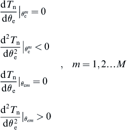 (11)
(11)
where
 (12)
(12)
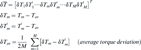
and where ![]() is a 2M dimensional vector given by:
is a 2M dimensional vector given by:
![]()
Figure 10.9 illustrates (qualitatively) the nonuniformity vector samples for a hypothetical torque waveform. Note that for perfectly uniform torque waveform ![]() with the result that n is a zm dimensional vector with all elements zero.
with the result that n is a zm dimensional vector with all elements zero.
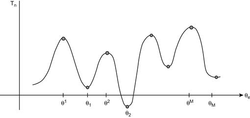
Figure 10.9 Illustrative torque waveform and its extrema.
The presence of a misfire can readily be detected by a scalar n derived from a norm of the vector ![]()
 (13)
(13)
The actual misfire detection is done on a statistical hypothesis testing basis. An experimental test of the misfire detection method was conducted in which there are three conditions expressed as hypothesis H0, H1, H2 where
H0 → normal engine operation
H1 → misfire in a single cylinder within an engine cycle
H2 → misfire in two cylinders within an engine cycle.
The tests were conducted on a four-cylinder engine having port fuel injection on each cylinder. The engine control system was programmed to interrupt fuel injection on one or two cylinders or on none. Instrumentation (explained later) was constructed which obtained the ![]() 1 norm of n (n1) for each of several thousand engine cycles. Figure 10.10 is a plot of the histogram for these data in which the distribution centered near
1 norm of n (n1) for each of several thousand engine cycles. Figure 10.10 is a plot of the histogram for these data in which the distribution centered near ![]() corresponded to H0. The distribution centered near
corresponded to H0. The distribution centered near ![]() corresponds to H1 and that centered near
corresponds to H1 and that centered near ![]() corresponds to H2. This histogram consists of the number of occurrences at the value n1 for each hypothesis Hi, N (n1, Hi) (i = 0, 1, 2) of nonuniformity index n1. The specific hypothesis under any test was determined by the number of cylinders that were caused to be misfired in the associated control instrumentation (i.e. 0, 1, 2 misfiring cylinders).
corresponds to H2. This histogram consists of the number of occurrences at the value n1 for each hypothesis Hi, N (n1, Hi) (i = 0, 1, 2) of nonuniformity index n1. The specific hypothesis under any test was determined by the number of cylinders that were caused to be misfired in the associated control instrumentation (i.e. 0, 1, 2 misfiring cylinders).
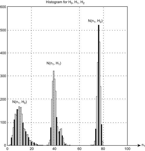
Figure 10.10 Histograms of nonuniformity index.
The detection of misfire can be based on a variety of criteria. For example, a simple statistical test can be a threshold comparison. Let Nav (H0) be the mean value for n1 under H0, Nav (H1) be the mean value for n1 under H1. A threshold nt is chosen such that
![]() (14)
(14)
The criterion for misfire is as follows:
n1 > nt → misfire
n1 < nt → no misfire.
There are two types of error associated with the above misfire criterion:
n1 < nt for an actual misfire (missed detection)
n1 > nt for no misfire (false alarm).
It should be noted that a similar statistical study was conducted using other threshold values. Choosing the threshold as done above yields approximately equal costs to both missed detection and false alarms.
The above method of detecting misfires does not, by itself, identify the cylinder(s) that is (are) misfiring. The nonuniformity index vector ![]() can be used as a further onboard diagnosis tool to assist the repair technician in identifying the misfiring cylinder(s). For an otherwise properly running engine a unique vector (
can be used as a further onboard diagnosis tool to assist the repair technician in identifying the misfiring cylinder(s). For an otherwise properly running engine a unique vector (![]() ) tends to be associated with the misfire in each cylinder. Assume initially that the above misfire detection indicates only a single cylinder is misfiring.
) tends to be associated with the misfire in each cylinder. Assume initially that the above misfire detection indicates only a single cylinder is misfiring.
The unique “signature” nonuniformity index for a consistent misfire in cylinder m will have nonuniformity vector ![]() . This “signature” can be obtained by running the engine with cylinder m purposely disabled (i.e. via fuel or spark). Data for the nonuniformity vector
. This “signature” can be obtained by running the engine with cylinder m purposely disabled (i.e. via fuel or spark). Data for the nonuniformity vector ![]() are given by the statistical average of
are given by the statistical average of ![]() over a sample of K engine cycles:
over a sample of K engine cycles:
 (15)
(15)
where ![]()
Each of these M vectors is directed to a point in a 2M dimensional space. The isolation of the misfiring cylinder is done by finding the shortest “distance” from a nonuniformity vector ![]() to these vectors. This vector distance (for the kth engine cycle) in 2M dimensional space
to these vectors. This vector distance (for the kth engine cycle) in 2M dimensional space ![]() is given by
is given by
![]() (16)
(16)
where ![]() is the measured nonuniformity vector for an engine cycle in which a single cylinder misfire has been detected. The problem of isolating the misfiring cylinder is reduced to finding the cylinder number mo, which yields the smallest
is the measured nonuniformity vector for an engine cycle in which a single cylinder misfire has been detected. The problem of isolating the misfiring cylinder is reduced to finding the cylinder number mo, which yields the smallest ![]() 2 norm for the vector distance
2 norm for the vector distance
![]() (17)
(17)
That is, cylinder mo (mo = 1, 2, … M) has the minimum ![]() and is identified as the misfiring cylinder.
and is identified as the misfiring cylinder.
If cylinder mo consistently misfires (as opposed to a random pattern) then by setting an appropriate flag in the diagnostic memory, the repair technician can know which cylinder should be analyzed for problems. This type of information greatly reduces the off-board diagnosis and maintenance effort. Often vehicles experience intermittent failures. A relatively simple onboard analysis program can evaluate the frequency of and the consistency of an intermittently misfiring cylinder.
Although the above method has great potential for detecting and diagnosing misfire problems, it cannot be directly implemented since there is no cost-effective method of measuring torque; however, the torque fluctuations δTn lead directly to crankshaft speed fluctuations which are measurable with a simple, inexpensive non-contacting sensor. We explain below the relationship between torque and crankshaft angular speed fluctuations. This relationship can be developed from a dynamic model for the power train as explained next.
A close enough estimate of δTn for misfire detection purposes can be obtained from a sliding mode observer (SMO) based upon a relatively straightforward system for measuring crankshaft angular speed (ωe). The model from which this SMO is built for an automatic transmission-equipped vehicle with unlocked torque converter is given below
![]() (18)
(18)
where J = moment of inertia of engine rotating parts
and where Tl = load torque on the engine output.
For the purposes of illustration, we consider the special case in which the vehicle is traveling under steady-state conditions for which Tl is a constant. This term can be neglected in the computation of torque fluctuations (as is done here).
Combining Eqns (10.4 through 10.8) with Eqn (10.18) yields the following model for ![]()
 (19)
(19)
The equations for Ti and TR have been given previously. Rewriting the above equation in state vector form with state vector x given by
![]()
![]() (20)
(20)
It is shown below that both x1 and x2 are measurable with inexpensive non-contacting sensors. Let the measurement of state vector x1 be denoted y1 and the measurement of x2 be denoted y2 The SMO for the estimate of x2 (which is denoted ![]() ) is given by:
) is given by:
 (21)
(21)
where ASMO = SMO gain
sgn( ) = sign function of argument.
The SMO gain requirement is that it be larger than the maximum value that can occur for (Pe − Po):
![]()
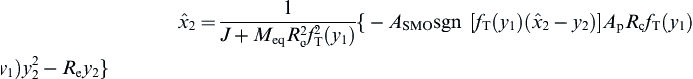
The estimate of indicated torque is obtained as the output of the first order filter given by
![]() (22)
(22)
![]()
Using this SMO to estimate ![]() it is possible to form δTn and the vector
it is possible to form δTn and the vector ![]() from which misfire detection is possible as explained above.
from which misfire detection is possible as explained above.
The measurement of crankshaft angular position and speed can readily be made using a non-contacting sensor such as that depicted in Figure 10.11 and as explained in Chapter 6. In Figure 10.11, the ferromagnetic disk (with lugs) is attached to the crankshaft. However, for the accuracy in measurements of θe and we required for SMO estimation of torque, there is a minimum number of lugs on the ferromagnetic disk. Experiments have shown that use of the starter ring gear which typically has 30-50 teeth is sufficient for these measurements.
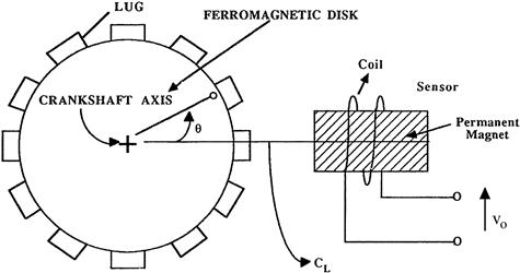
Figure 10.11 Non-contacting crankshaft angular speed sensor.
For illustrative purposes it is convenient to consider these measurements at a relatively slowly changing RPM. In this case the crankshaft angular speed ωe(t) is given by:
![]() (23)
(23)
δωe(t) = variation in ωe due to δTn
This angular speed is actually in the form of a frequency-modulated (FM) carrier frequency in which Ωe acts as the carrier frequency and δωe(t) is the modulation. It should be noted that Ωe ![]() max (δωe).
max (δωe).
The crankshaft instantaneous angular position θe(t) is given by
 (24)
(24)
where θo = θe(0) = phase reference.
The phase reference can be established relative to the engine cycle via a camshaft once/revolution non-contacting sensor (see Chapter 7).
The sensor output signal v0(t) is given by
![]() (25)
(25)
where Md = number of lugs on disk
ψ(t) = random process (error in the sensor output).
The function f(·) is the waveform associated with the sensor configuration. Fortunately the electronic signal processing required to measure ωe(t) can be obtained using either analog or digital electronic signal processing. Figure 10.12 shows a block diagram for an analog signal processing.
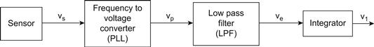
Figure 10.12 Block diagram for ωe measurement.
The “frequency to voltage converter” is in effect an FM demodulator which can be implemented with a circuit known as a “phase-locked loop” (PLL). The PLL is an electronic closed-loop system. It is output voltage vp(t) is given by
![]()
The low-pass filter (LPF) passes the first term and suppresses that portion of the spectrum of ![]() which lies outside the LPF pass bands thereby yielding the measurement of ωe needed for the SMO to compute
which lies outside the LPF pass bands thereby yielding the measurement of ωe needed for the SMO to compute ![]() . For the present analysis it is assumed that this portion of
. For the present analysis it is assumed that this portion of ![]() is negligible. The crankshaft angular position can be obtained by integrating the LPF output voltage. Using the integrator circuit described in Chapter 3 the integrator output voltage VI is given by
is negligible. The crankshaft angular position can be obtained by integrating the LPF output voltage. Using the integrator circuit described in Chapter 3 the integrator output voltage VI is given by
![]() (26)
(26)
where τi = integrator time constant
Of course, digital integration as explained previously (e.g. see Chapter 8) can also be used to obtain VI. The phase origin for this measurement of θe(t) is established via the once/revolution camshaft sensor. The measurement of θe is required as part of the computation of the nonuniformity index ![]() .
.
In a contemporary implementation the measurement of ωe(t) is done in discrete time based upon successive samples of vo(t). As explained in Chapter 6, a sensor such as is depicted in Figure 10.12 generates an output waveform which crosses zero whenever one of the lugs on the disk lies along the centerline (CL) of the disk sensor axis. Let tk be the time of the kth zero crossing of the sensor output voltage, and let δtk be given by:
![]()
The kth sample of ωe(t) which is denoted ωe(k) and is given by:
![]() (27)
(27)
If Md is sufficiently large, the sequence {ωe(k)} will be an un-aliased sample of ωe(k).
The instantaneous crankshaft angular position θe(k) is given by:
![]() (28)
(28)
This sampled crankshaft angular position is readily obtained by passing the sensor through a zero crossing detector (ZCD) and counting the output pulses using a binary counter (see Chapter 4 for an explanation of a counter) as explained in Chapter 6. The counter should be reset by a signal from the once/revolution camshaft sensor. This signal is also sent to a ZCD and then to the binary counter reset input. This configuration will automatically count zero crossings of the crankshaft sensor of Figure 10.12 modulo 2Md.
Using the instrumentation above for measuring ωe and θe provides the necessary values for a calculation of ![]() using the SMO as well as the nonuniformity index
using the SMO as well as the nonuniformity index ![]() . The misfire detection proceeds using the estimate of Tn according to the procedure explained earlier.
. The misfire detection proceeds using the estimate of Tn according to the procedure explained earlier.
The above hypothetical method of misfire detection has been shown to reliably detect misfires both in a laboratory environment and in actual road tests. For a test vehicle equipped with an automatic transmission total errors of less than 1% have been achieved for the exemplary misfire detection in actual road tests. Although intellectual property considerations preclude discussing the actual misfire detection methods used by any automotive manufacturer, many of the components of the hypothetical system are to be found in some of them.
Expert Systems in Automotive Diagnosis
An expert system is a computer program that employs human knowledge to solve problems normally requiring human expertise. The theory of expert systems is part of the general area of computer science known as artificial intelligence (AI). The major benefit of expert system technology is the consistent, uniform, and efficient application of the decision criteria or problem-solving strategies. We consider next a hypothetical expert system devoted to automotive diagnosis.
The diagnosis of electronic engine control systems by an expert system proceeds by following a set of rules that embody steps similar to the diagnostic charts in the shop manual. The diagnostic system can receive fault codes from the onboard diagnostic. The system processes these codes logically under program control in accordance with the set of internally stored rules. However, as explained above, not all faults are detected by the onboard diagnostic system. Testing of various systems and components by the service technician as directed by the expert system aids the diagnosis of problems. The hypothetical expert system-based diagnostic procedure also is designed to receive inputs from the service technician based on such tests. The end result of the computer-aided diagnosis is an assessment of the problem and recommended repair procedures. The use of an expert system for diagnosis has the potential to improve the efficiency of the diagnostic process and can thereby reduce maintenance time and costs.
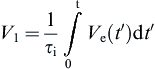
The development of an expert system requires a computer specialist who is known in AI parlance as a knowledge engineer. The knowledge engineer must acquire the requisite knowledge and expertise for the expert system by interviewing the recognized experts in the field. In the case of automotive electronic engine control systems the experts include the design engineers, the test engineers and technicians, involved in the development of the control system. In addition, expertise is developed by the service technicians who routinely repair the system in the field. The expertise of this latter group can be incorporated as evolutionary improvements in the expert system. The various stages of knowledge acquisition (obtained from the experts) are outlined in Figure 10.13.
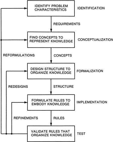
Figure 10.13 Expert system development procedure.
It can be seen from this illustration that several iterations are required to complete the knowledge acquisition. Thus, the process of interviewing experts is a continuing process.
Not to be overlooked in the development of an expert system is the personal relationship between the experts and the knowledge engineer. The experts must be fully willing to cooperate and to explain their expertise to the knowledge engineer if a successful expert system is to be developed. The personalities of the knowledge engineer and experts can become a factor in the development of an expert system.
Figure 10.14 represents the environment in which an expert system evolves. Of course, a digital computer of sufficient capacity is required for the development work. A summary of expert system development tools that have been used in the past and that are potentially applicable for a mainframe computer is presented in Table 10.2.
Figure 10.14 Environment of an expert system.
Table 10.2 Expert system developing tools for mainframes.
| Name | Company | Machine |
| Ops5 | Carnegie Mellon University | VAX |
| S.1 | Teknowledge | VAX |
| Xerox 1198 | ||
| Loops | Xerox 1108 | |
| Kee | Intelligenetics | Xerox 1198 |
| Art | Inference | Symbolics |
It is common practice to think of an expert system as having two major portions. The portion of the expert system in which the logical operations are performed is known as the inference engine. The various relationships and basic knowledge are known as the knowledge base.
The general diagnostic field to which an expert system is applicable is one in which the procedures used by the recognized experts can be expressed in a set of rules or logical relationships. The automotive diagnosis area is clearly such a field. The diagnostic charts that outline repair procedures (as outlined earlier in this chapter) represent good examples of such rules.
To clarify some of the ideas embodied in an expert system, consider the following example of the diagnosis of an automotive repair problem. This particular problem involves failure of the car engine to start. It is presumed in this example that the range of defects is very limited. Although this example is not necessarily commonly encountered, it does illustrate some of the principles involved in an expert system.
The fundamental concept underlying this example is the idea of condition-action pairs that are in the form of IF-THEN rules. These rules embody knowledge that is presumed to have come from human experts (e.g. experienced service technicians or automotive engineers).
A typical expert system formulates expertise in IF-THEN rules.
The expert system of this example consists of three components:
Each rule of the rule base is of the form of “if condition A is true, then action B should be taken or performed.” The IF portion contains conditions that must be satisfied if the rule is to be applicable. The THEN portion states the action to be performed whenever the rule is activated (fired).
The database contains all the facts and information that are known to be true about the problem being diagnosed. The rules from the rule base are compared with the knowledge base to ascertain which are the applicable rules. When a rule is fired, its actions normally modify the facts within the database.
The controlling mechanism of this expert system determines which actions are to be taken and when they are to be performed. The operation follows four basic steps:
(1) Compare the rules to the database to determine which rules have the IF portion satisfied and can be executed. This group is known as the conflict set in AI parlance.
(2) If the conflict set contains more than one rule, resolve the conflict by selecting the highest priority rule. If there are no rules in the conflict set, stop the procedure.
(3) Execute the selected rule by performing the actions specified in the THEN portion, and then modify the database as required.
(4) Return to Step 1 and repeat the process until there are no rules in the conflict set.
In the present simplified example, it is presumed that the rule base for diagnosing a problem starting a car is as given in Figure 10.15.

Figure 10.15 Simple automobile diagnostic rule base.
Rules R2 through R7 draw conclusions about the suspected problem, and rule R1 identifies problem areas that should be investigated. It is implicitly assumed that the actions specified in the THEN portion include “add this fact to the database.” In addition, some of the specified actions have an associated fractional number. These values represent the confidence of the expert who is responsible for the rule that the given action is true for the specified condition.
Further suppose that the facts known to be true are as shown in Figure 10.16.

Figure 10.16 Starting database of known facts.
The controlling mechanism follows Step 1 and discovers that only R1 is in the conflict set. This rule is executed, deriving these additional facts in performing Steps 2 and 3:
At Step 4, the system returns to Step 1 and learns that the conflict set includes R1, R4, and R6. Since R1 has been executed, it is dropped from the conflict set. In this simplified example, assume that the conflict is resolved by selecting the lowest numbered rule (i.e. R4 in this case). Rule R4 yields the additional facts after completing Steps 2 and 3 that there is a break in the fuel line (0.65). The value 0.65 refers to the confidence level of this conclusion.
The procedure is repeated with the resulting conflict set R6. After executing R6, the system returns to Step 1, and finding no applicable rules, it stops. The final fact set is shown in Figure 10.17. Note that this diagnostic procedure has found two potential diagnoses: a break in the fuel line (confidence level 0.65), and mixture too rich (confidence level 0.70).
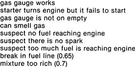
Figure 10.17 Final resulting database of known facts.
The previous example is intended merely to illustrate the application of AI to automotive diagnosis and repair. To perform diagnosis on a specific car using an expert system, the service technician identifies all the relevant features to the service technician’s terminal including, of course, the engine type. After connecting the data link from the onboard diagnostic system to the terminal, the diagnosis can begin. The terminal can ask the service technician to perform specific tasks that are required to complete the diagnosis, including, for example, starting or stopping the engine.
The expert system is an interactive program and, as such, has many interesting features. For example, when the expert system requests that the service technician perform some specific task, he/she can ask the expert system why he or she should do this, or why the system asked the question. The expert system then explains the motivation for the task, much the way a human expert would do if he or she were guiding the service technician. An expert system is frequently formulated on rules of thumb that have been acquired through years of experience by human experts. It often benefits the service technician in his or her task to have requests for tasks explained in terms of both these rules and the experience base that has led to the development of the expert system.
The general science of expert systems is so broad that it cannot be covered in this book. The interested reader can contact any good engineering library for further material in this exciting area. In addition, the SAE has many publications covering the application of expert systems to automotive diagnosis.
From time to time, automotive maintenance problems will occur that are outside the scope of the expertise incorporated in the expert system. In these cases, an automotive diagnostic system needs to be supplemented by direct contact of the service technician with human experts. Automobile manufacturers all have technical assistance available to service technicians via internal connections, or e-mail.
Vehicle off-board diagnostic systems (whether they are expert systems or not) continue to be developed and refined as experience is gained with the various systems, as the diagnostic database expands, and as additional software is written. The evolution of such diagnostic systems may be heading in the direction of fully automated, rapid, and efficient diagnoses of problems in cars equipped with modern digital control systems.
Occupant Protection Systems
Occupant protection during a crash has evolved dramatically since about the 1970s. Beginning with lap seat belts, and motivated partly by government regulation and partly by market demand, occupant protection has evolved to passive restraints and airbags. We will discuss only the latter since airbag deployment systems can be implemented electronically, whereas other schemes are largely mechanical. Whereas the first airbag occupant protection systems were intended for occupant protection in crashes that were mostly along the vehicle longitudinal axis, contemporary vehicles provide side impact protection.
Occupant protection by an airbag is conceptually quite straightforward. The airbag system has a means of detecting when a crash occurs that is essentially based on exceptional deceleration along a car axis. A collision that is serious enough to injure car occupants involves deceleration in the range of tens or hundreds of gs, whereas normal driving involves acceleration/deceleration less than 1 g.
Once a crash has been detected, a flexible bag is rapidly inflated with a gas that is released from a container by electrically igniting a chemical compound. Ideally, the airbag inflates in sufficient time (e.g. typically ≤50 ms) to act as a cushion for the driver (or passenger) as he or she is thrown forward or sideways during the crash.
On the other hand, practical implementation of the airbag has proven to be technically challenging. At car speeds that can cause injury to the occupants, the time interval for a crash into a rigid barrier from the moment the front bumper contacts the barrier until the final part of the car ceases forward motion is of the order of a second. Table 10.3 lists required airbag deployment times for a variety of test crash conditions.
Table 10.3 Airbag deployment times.
| Test Library Event | Required Deployment Time (ms) |
| 9 mph frontal barrier | ND |
| 9 mph frontal barrier | ND |
| 15 mph frontal barrier | 50.0 |
| 30 mph frontal barrier | 24.0 |
| 35 mph frontal barrier | 18.0 |
| 12 mph left angle barrier | ND |
| 30 mph right angle barrier | 36.0 |
| 30 mph left angle barrier | 36.0 |
| 10 mph center high pole | ND |
| 14 mph center high pole | ND |
| 18 mph center high pole | ND |
| 30 mph center high pole | 43.0 |
| 25 mph offset low pole | 56.0 |
| 25 mph car to car | 50.0 |
| 30 mph car to car | 50.0 |
| 30 mph 550 hop road, panic stop | ND |
| 30 mph 629 hop road, panic stop | ND |
| 30 mph 550 tramp road, panic stop | ND |
| 30 mph 629 tramp road, panic stop | ND |
| 30 mph square block road, panic stop | ND |
| 40 mph washboard road, medium braking | ND |
| 25 mph left-side pothole | ND |
| 25 mph right-side pothole | ND |
| 60 mph chatter bumps, panic stop | ND |
| 45 mph massoit bump | ND |
| 5 mph curb impact | ND |
| 20 mph curb drop-off | ND |
| 35 mph Belgian blocks | ND |
Note: ND = nondeployment.
A typical airbag will require about 30 ms to inflate, meaning that the crash must be detected within about 20 ms. With respect to the speed of modern digital electronics, a 20-ms time interval is not considered to be short. The complicating factor for crash detection is the many crash-like accelerations/decelerations experienced by a typical car that could be interpreted by airbag electronics as a crash, such as impact with a large pothole or driving over a curb.
The configuration for an airbag system has also evolved from electromechanical implementation (using switches) to electronic systems employing sophisticated signal processing. One of the early configurations that was intended to protect occupants from longitudinal axis deceleration employed a pair of acceleration switches SW1 and SW2 as depicted in Figure 10.18. Each of these switches is in the form of a mass suspended in a tube with the tube axis aligned parallel to the longitudinal car axis. Figure 10.18b is a circuit diagram for the airbag system.
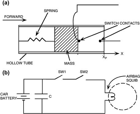
Figure 10.18 Airbag deployment system.
The two switches, which are normally open, must both be closed to complete the circuit for firing the airbag. When this circuit is complete, a current flows through the ignitor that activates the charge. A gas is produced (essentially explosively) that inflates the airbag.
The switches SW1 and SW2 are placed in two separate locations in the car. Typically, one is located near the front of the car and one in or near the front of the passenger compartment (some automakers locate a switch under the driver’s seat on the floor pan).
Referring to the sketch in Figure 10.18, the operation of the acceleration-sensitive switch can be understood. Under normal driving conditions the spring holds the movable mass against a stop and the switch contacts remain open. During a crash the force of acceleration (actually deceleration of the car) acting on the mass is sufficient to overcome the spring force and move the mass. For sufficiently high car deceleration, the mass moves forward to close the switch contacts. In a real collision at sufficient speed, both switch masses will move to close the switch contacts, thereby completing the circuit and igniting the chemical compound to inflate the airbag.
An approximate dynamic model for the mechanical crash sensor is given below:
![]() (29)
(29)
where M = mass of the movable element
D = viscous friction coefficient
Fc = coulomb friction force (stiction)
K = spring constant.
x = mass displacement of M from stop.
The acceleration of the mass (![]() ) is related to vehicle acceleration a or deceleration (−a) by the following
) is related to vehicle acceleration a or deceleration (−a) by the following
![]()
The motion of the movable mass is the solution to the following:
![]() (30)
(30)
Whenever the mass displacement exceeds the spacing to the switch contact (xp) (i.e. x = xp) the contacts close and the action described above proceeds.
Figure 10.18 also shows a capacitor connected in parallel with the battery. This capacitor is typically located in the passenger compartment. It has sufficient capacity that in the event the car battery is destroyed early in the crash, it can supply enough current to ignite the squib.
In recent years, there has been a trend to implement electronic airbag systems. In such systems the role of the acceleration-sensitive switch is played by an analog accelerometer along with electronic signal processing, threshold detection, and electronic driver circuit to fire the squib. Figure 10.19 depicts a block diagram of such a system.
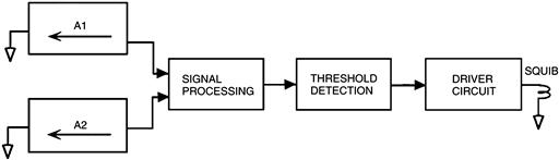
Figure 10.19 Accelerometer-based airbag system.
The accelerometers A1 and A2 are placed at locations similar to where the switches SW1 and SW2 described above are located. Each accelerometer outputs a signal that is proportional to acceleration (deceleration) along its sensitive axis. As an illustration of the characteristic waveform from an accelerometer, Figure 10.20 presents measurements of a 3200 lb (curb weight) vehicle that was crashed into a rigid barrier at 30 mph.
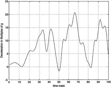
Figure 10.20 Acceleration data for 30 mph crash.
Under normal driving conditions, the acceleration at the accelerometer locations is less than 1 g. However, during a collision at a sufficiently high speed the signal increases rapidly. Signal processing can be employed to enhance the collision signature in relation to the normal driving signal. Such signal processing must be carefully designed to minimize time delay of the output relative to the collision deceleration signal. A comparison of the deceleration profile of Figure 10.20 for this crash with the deployment requirements of Table 10.3 illustrates the complexity of the signal processing necessary to properly deploy the airbag.
After being processed, the deceleration signal is compared with a threshold level. As long as the processed signal is less than this threshold the driver circuit remains deactivated. However, when this signal exceeds the threshold, the driver circuit sends a current of sufficient strength to activate the chemical and inflate the airbag.
Typically, the threshold is set so that airbag deployment occurs for a crash into a barrier at or above a specific speed. Depending on the system design, this speed can be anywhere between 8 and 12 mph. This speed range is chosen by the manufacturer to optimize the protection offered to the car occupants while minimizing (or completely eliminating) false deployment (that is, deployment when there is no crash).
In addition to airbags for protecting the driver and front seat passenger against frontal collision, airbags have become available for occupant protection against other types of collisions. Airbags now are available for protection against side impact. Conceptually, these occupant protection systems operate in ways similar to the type described above.
There will continue to be new developments in airbag technology in order to improve performance. Complicating this task is the fact that the signature of a crash differs depending on the crash configuration and vehicle design. For example, there is one class of signature for a crash into a rigid barrier (i.e. a nonmoving and incompressible object) and another for a crash between a pair of cars (particularly when vehicle curb weights are different). In spite of technical difficulties in implementation, the airbag is finding broad application for occupant protection and has achieved broad acceptance by the driving public.
In addition to airbags, contemporary vehicles employ passive restraint systems consisting of lap and over-the-shoulder belts. These passive restraints combined with airbags offer a high level of occupant protection. Although it is not an electronic system, another aspect of occupant protection comes from an optimal vehicle structural design. Contemporary vehicles are structurally designed to absorb crash energy in such a way as to minimize intrusion of damage into the passenger compartment.