4	Digital TV by Satellite
CHAPTER

FIGURE

    4.1

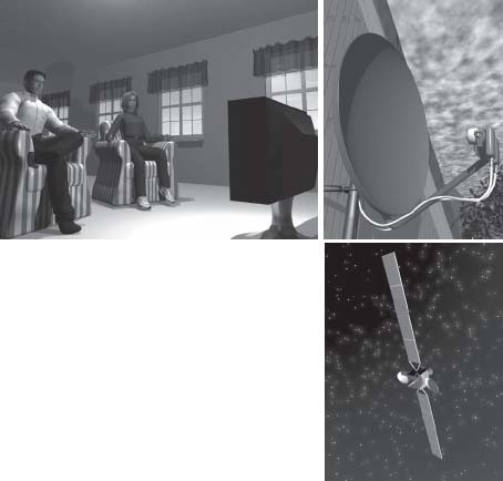
Satellite TV opens up window to the world outside.

The previous chapter described how the geostationary satellites distribute TV and radio channels using beams of microwave radio waves covering extensive areas on the Earth's surface. We will now move down to Earth and see how we can make use of the satellite signals.

SATELLITE POSITIONS AND POWER

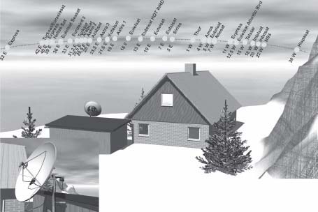
Seen from ground, the geostationary orbit looks like a curve in the southern sky that extends from east to west (see Figure 4.2). From a location at the equator the orbit looks like a line straight across the sky. The orbital position that corresponds to the longitude of the location is straight up. The part of the geostationary orbit that is visible from the central parts of Europe is approximately between 60 degrees west and 90 degrees east, depending on location. This is 150 degrees of the 360 degree geostationary orbit. Orbital positions further to the west or further to the east are closer to the horizon and harder to receive. Positions even further away fall below the horizon. Orbital positions can be placed at a distance of three degrees apart, so about 50 orbital positions may be located within the visible part of the orbit.

The maximum angular height, elevation angle, of the geostationary satellites varies between 45 degrees in the southern parts of Europe and 10 degrees in the most northern parts.

FIGURE

    4.2

The geostationary orbit extends from east to west in the southern sky. Here some of the more important European orbital positions are shown.

FINDING THE SATELLITE

We will soon return to the parabolic dish and what happens after that the signal has been concentrated at the focus. But first we will take a closer look at what it takes to point the antenna right towards the desired satellite.

When I first started working with satellite TV, more than 20 years ago, it was more or less a mystery to find a satellite. It was hard to calculate where in the sky the satellite really was. Today nobody has to care about that, because there are maps showing where in the sky to find a specific satellite wherever you are. As soon as you know the angles toward the satellite, the next step is to apply them in practice to the antenna.

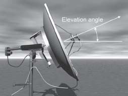
Elevation Angle

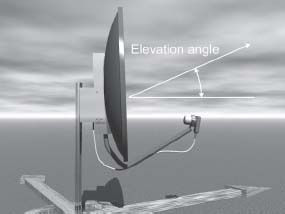
The first angle is the angle of elevation to the satellite. This angle is the height of the satellite in degrees (see Figure 4.3). In the old days, it was easy to decide the angle of elevation for the center-feed parabolic dish most common then. The boresight direction of center-feed antenna is at right angles relative to the edge of the aperture of the dish (see Figures 4.2 and 4.36).

FIGURE

    4.3

The elevation angle defined (offset antenna).

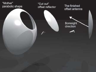
Today, most parabolic antennas are of the offset kind. These antennas are created by a segment being cut out from a deep parabolic surface, as in Figure 4.4.

FIGURE

    4.4

The offset antenna is created by a section being cut out from a deep parabolic surface.

The result is an antenna that does not have a symmetrical profile, making it hard to know the boresight direction of the antenna. The boresight direction of the antenna is the view direction of the antenna, the direction in which the antenna is most sensitive. The manufacturer might have put a scale or some kind of reference plane on the antenna identifying the elevation angle. The mount of the antenna has to be mounted absolutely vertically to ensure a correct angle based on the scale provided. (This is easily done with a water level or a weighted string.)

Azimuth Angle

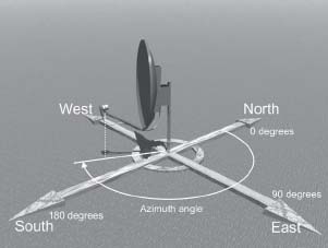
The other angle that we need to know is the azimuth angle of the antenna. The azimuth angle is the angle between north and the location of the satellite. This is always counted clockwise. Figure 4.5 shows that a satellite located straight to north has an azimuth angle of 0 degrees, to the east has an azimuth angle of 90 degrees, to the south is 180 degrees and west is 270 degrees.

FIGURE

    4.5

The azimuth angle defined.

A satellite positioned at a longitude that is more to the east than the longitude of the receiving site has an azimuth angle that is less than 180 degrees. A satellite positioned to the west of the reception site has an azimuth angle that is greater than 180 degrees.

Note

A common error is caused by people using compasses that have 400 degrees instead of 360 degrees when searching for satellites. In the satellite business, all angles are based on 360 degrees.

Even if you know the elevation and azimuth angles, it is not really that easy to find the satellites. It is also quite hard to transfer the azimuth angle to an antenna in practice. It is quite hard to know the point of the compass with any accuracy. Compasses only provide an approximate direction towards the north and are disturbed by metal objects that are close by.

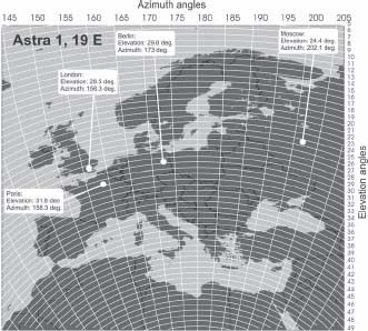
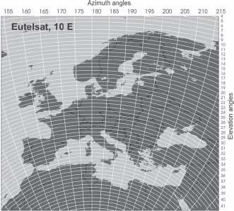
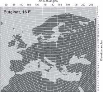
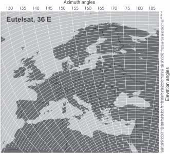
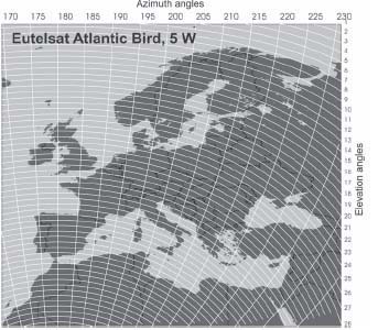
Figures 4.6 through 4.17 are elevation and azimuth maps for some important European orbital positions. Elevations angles are read to the right and azimuth angles are on top. First is SES Astra, a part of SES Global, that operate satellites at three major orbital positions; 19 degrees east, 28.5 degrees east and 23.5 degrees east.

FIGURE

    4.6

The main position of Astra at 19 degrees east, elevation and azimuth angles.

FIGURE

    4.7

SES Astra's second orbital position is at 28 degrees east.

FIGURE

    4.8

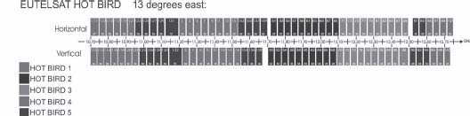
The most Eutelsat's most important orbital position is the HOT BIRD position at 13 degrees east.

FIGURE

    4.9

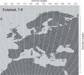
Eutelsat's orbital position at 7 degrees east.

FIGURE

  4.10

Eutelsat's orbital position at 10 degrees east.

FIGURE

  4.11

The Eutelsat orbital position at 16 degrees east.

FIGURE

  4.12

The Eutelsat orbital position at 36 degrees east.

FIG

  4.13

The Eutelsat Atlantic Bird orbital position at 5 degrees west.

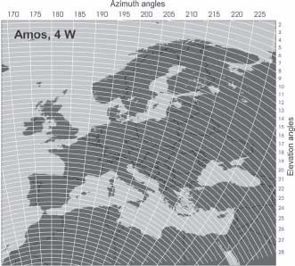
FIG

  4.14

The Amos orbital position at 4 degrees west.

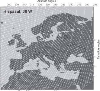
FIGURE

  4.15

Farther west, we find the Spanish Hispasat system.

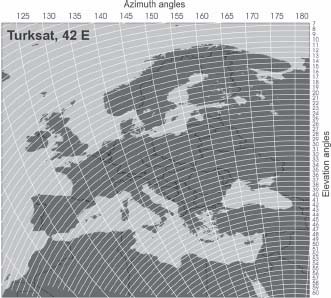
FIGURE

  4.16

Farther east, we have one of the Turkish Turksat orbital positions.

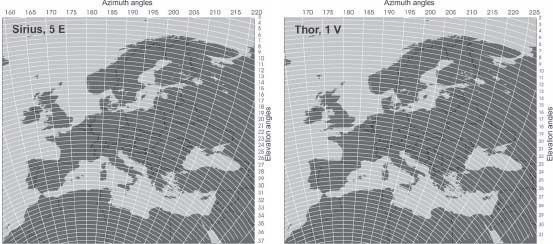
FIGURE

  4.17

The “Sirius” and the “Thor” satellite systems are Scandinavian regional satellite systems that also have European coverage areas.

POSITIONING THE DISH

When installing a parabolic dish, a free line of sight to the satellite is a necessity. Sometimes there might be obstacles such as trees or buildings, and it may be hard to know if there is a free line of sight towards the satellite. But with the elevation and azimuth angles, it is possible to check the visibility to the satellite. The main problem is determining the antenna location without having the actual antenna in place for testing.

There are special aiming compasses which are a great help for testing the visibility. The Suunto compass is primarily intended for the lumbering industry in order to be able to measure the height of a tree without first having to cut it down but is a handy tool for determining the proper placement of satellite dishes.

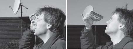
FIGURE

  4.18

There are professional instruments for finding the satellites, but you can also build your own.

Another cheaper alternative is using a protractor and a weighted string. If you look along the protractor, as in Figure 4.18, you can check the visibility at a certain elevation angle.

The trick of quickly finding the right satellite when pointing the dish is starting with the elevation angle. This angle is easier than the azimuth angle to determine, since a weighted string or a water level easily determines an exact vertical line. From this line, the exact angle of elevation can be measured. This measurement is easier if there is an integrated scale for the elevation angle in the antenna design. If there is no such scale, there might be a plane of reference in relation to which the true elevation angle is known. Check for that in the installation manual for the antenna.

Since the angle within which a satellite dish is sensitive is very narrow, it is hard to find the correct angle towards the satellite. You should first point the antenna in approximately the right direction to give yourself a better chance to actually look for the signal.

When you believe the antenna is pretty close to the right elevation angle, the next step is to search for the satellite by adjusting the azimuth angle and hopefully the satellite signals will show up.

By starting with the elevation angle, you avoid the tough task of establishing a true north-to-south line, which is necessary for deciding the azimuth angle prior to installation. And even if this direction is accurately known, it is almost impossible to use this knowledge to accurately point the antenna, because it is hard to transfer the direction to the antenna itself. Since you can attach a weighted string directly to the antenna, it is much easier to get to know the true elevation angle and to read the actual azimuth angle.

Satellite signals are really very weak. A typical satellite transponder has an output power of less than 100 Watts. This is comparable to the power consumption of an ordinary light bulb. The power is spread across an area that might be as large as Europe. Still, it is possible to receive the signals using a relatively small antenna. A parabolic dish with a diameter of 90 centimeters has an area of barely 0.65 square meters. Compared to the surface of Europe, the signal power collected by the dish is almost nothing; in technical terms, it is in the range of pikowatts, i.e., 0.000000000001 watt (12 decimals).

To handle the extremely low signal levels, we first have to collect all power that gets into the antenna. The easiest way of doing so is by using a parabolic reflector that optically concentrates the signal towards its focal point (see Figure 4.19). A lot of the power that hit the antenna could be found in the focus. However there are losses that reduce the amount of useable power to about 55 to 75 percent.

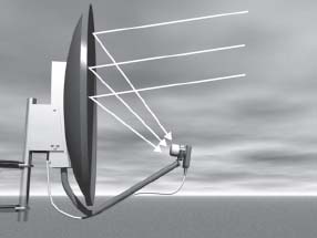
FIGURE

  4.19

The parabolic dish concentrates the incoming power to one point, the focus.

LOW NOISE BLOCK CONVERTERS (LNBS)

When the received signal power has been concentrated in the focal point of the reflector, it has to be collected and treated further. The dish focus contains a Low Noise Block converter (LNB). There are three tasks for the block converter: amplify the weak signal, down-convert it into a lower frequency range, and choose polarization and what part of the frequency range that is to be received. The reason the signals have to be down converted is because microwave high frequency signals are attenuated too much to be transported to the receiver.

Inside the LNB, there are two small antennas about a quarter of a wavelength long. This would mean about 6 millimeters (in the 12 GHz band the wavelength is about 2.5 centimeters). The antennas are oriented at right angles to each other so that one receives the horizontal signals while the other receives the vertical. The antennas are followed by a low noise amplifier that usually consists of two low noise transistors.

The low noise transistors amplify the signal to about 20 dB, corresponding increasing the signal power level by 100 times. Now the signal goes to a mixer where it is mixed with a locally generated oscillator signal. After the mixer, a new signal is obtained that has the frequency which corresponds to the difference between the incoming signal and the local oscillator signal.

The LNB takes care of a complete “block” of frequencies that are amplified and converted to a lower frequency range. In the childhood days of satellite TV, there were low noise converters that could receive signals from just one transponder. Being able to receive a larger frequency range was a real sensation in those days and there was a demand for a “block” converter.

The down-converted signals coming from the mixer are amplified by an additional 30 dB (1,000 times) by two or three other transistors before the signal is fed to the indoor satellite receiver.

Universal LNB

SES Astra saw the need for an LNB with a large input frequency range and suggested an LNB covering the whole range from 10.70 to 12.75 GHz. This is called the Universal LNB. To use the whole range, the frequency range has to be divided into two parts. The lower part is 10.70 to 11.70 GHz and the upper part is 11.70 to 12.75 GHz. As described above, a signal can be down-converted to a lower frequency by being mixed with a locally generated signal, the local oscillator signal. The down-converted signal is found at a frequency that is the difference between the frequency of the incoming signal and the local oscillator frequency.

If the frequencies in the lower frequency band are mixed with a local oscillator of 9.75 GHz, the difference with the signals of the incoming signals in the 10.70 to 11.70 GHz band will be signals in the frequency range of 0.95–1.95 GHz. Just the same, when the incoming signals are in the upper frequency band, 11.70-12.75 GHz, and the local oscillator frequency is 10.60 GHz, the difference between the signals will be between 1.10 and 2.15 GHz. Therefore, the LNB has to be able to switch between two local oscillator frequencies: 9.75 and 10.60 GHz.

Another result is that, a universal LNB will generate output signals in the range of 950 to 2150 MHz. This frequency range is called the satellite intermediate frequency band, or the L-Band, and is used to transport the signals from the LNB to the satellite receiver that is placed close to the TV set.

When a 22 kHz tone is sent from the receiver on the cable, the upper frequency range should be received and the LNB is switched to the 10.60 GHz local oscillator. With no tone on the cable, the lower frequency range should be received and the 9.75 GHz local oscillator should be in operation.

On top of this, the receiver must also be able to switch between vertical and horizontal polarization by switching between the two small antennas in the feed horn of the LNB. A way of doing this is by changing the supply voltage to the LNB between 14 volts for the vertical polarization and 18 volts for the horizontal polarization.

In order to be called a universal LNB, there is still one more requirement to fulfill. The LNB also must be able to receive digital, phase-modulated signals.

Finally the distance between the parabolic dish and the receiver should not exceed more than between 20 and 30 meters (70 to 100 feet). If this distance is exceeded, thicker cables or line extending amplifiers (line extenders) might be needed.

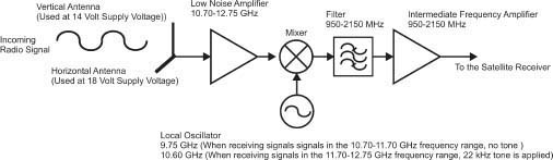
FIGURE

  4.20

The principal design of a universal LNB.

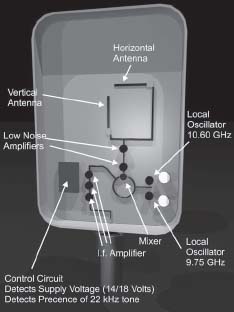
FIG

  4.21

The interior of a universal LNB.

THE SATELLITE RECEIVER

The satellite receiver is an indoor device that receives signals in the frequency range of 950 to 2150 MHz (also called the L-Band). Since satellite TV is a truly multi-channel media, the receiver must be equipped with a processor and software that is capable of handling all the channels. This processor also controls the supply voltage to the LNB as well as the presence or absence of the 22 kHz tone. This controls the frequency range of the LNB to receive the TV channel requested by the viewer.

When the signal from the LNB enters the satellite receiver, it is first handled by the input stage, the tuner. The main purpose of the tuner is to select which transponder is to be received. To be able to do this, the tuner also has to send the right supply voltage to obtain signals of the right polarization, as well as supply the 22 kHz tone if the requested transponder is located in the upper part of the frequency band (11.70–12.75) GHz. The most important thing, however, is that the tuner chooses a more limited frequency range around the selected transponder and down-converts the signal further to a second intermediate frequency around 480 MHz. At this frequency, there is a filter that has a bandwidth of about 30 MHz (approximately corresponding to the bandwidth of a transponder).

Now the desired carrier containing the content in the requested transponder is sent on to the demodulator. The demodulator's job is to recover the digital bit stream of the digital DVB-S multiplex. In digital satellite TV, the most common kind of modulation is Quadrature Phase Shift Keying (QPSK). In this modulation scheme, the radio wave alternates between four different phase angles.

When the signal is demodulated and the original transport stream has been recovered, the next step is to demultiplex the transport stream to find the audio, video and teletext packets that belong to the selected TV channel. Last, these packets are sent to the audio and video decoder respectively. The rest of the process has already been described in Chapter 2.

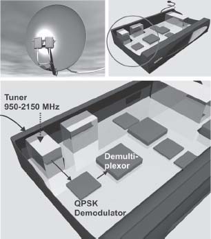
FIGURE

  4.22

In the satellite receiver there is an input stage, the tuner, covering the frequency range 950–2150 MHz. This is followed by a demodulator capable of handling Quadrature Phase Shift Keying, QPSK.

MODULATING DIGITAL SIGNALS

Radio waves are electromagnetic waves that are created when electrons are moving forth and back in an electrical conductor. All radio waves originate in electrical oscillator circuits. If you wish to build an electrical oscillator, you can take the output signal of an amplifier and connect it to the input of the same amplifier, which will make the amplifier oscillate. If the oscillating amplifier is connected to an electric conductor, the electrons inside the conductor start to oscillate as well. But when electrical charges (as the electrons are) begin to move forth and back, electromagnetic waves start to propagate from the conductor.

When this radio wave hits another electrical conductor, the electrons in this conductor also start to move forth and back following the same pattern as in the “transmitting” conductor.

We have succeed in transferring the movement of electrons in the transmitting conductor (antenna) to the electrons in the receiving (conductor) in a completely wireless way.

However there is no reason to transfer this movement of electrons if there is no message carried by the radio wave. What we want to do is to use the radio wave as a carrier of information, a carrier wave.

Amplitude Modulation

The first technology for getting the wave to carry information was amplitude modulation, AM. AM is based on letting the strength or the amplitude of the radio wave vary in line with the signal containing the information that we want to transfer.

AM has been in use since the beginning of the twentieth century but has some critical drawbacks.

Amplitude modulation does not require that much bandwidth but on the other hand is quite sensitive to disturbances. Therefore AM requires quite a lot of transmission power in order to suppress noise and interference. AM has been used for transmission of the video in the analogue terrestrial TV networks.

Frequency Modulation

A better analog way of modulation is frequency modulation, FM. Frequency modulation is based on varying the frequency of the carrier wave in line with the message signal that is to be transferred. FM has a better resistance to noise and interference but also occupies more bandwidth than AM. In analog satellite transmissions of TV, frequency modulation has been used, because bandwidth is less expensive than transmission power.

Phase Modulation

When carrying digital signals, we only have to carry two messages, the digits “0” and “1.” Therefore there are other more efficient ways to modulate a carrier wave than using AM or FM. The third way of modulation is phase modulation, PM. Phase modulation is achieved by letting the wave make a phase jump, as in Figure 4.23. In the simplest phase modulation scheme, the wave jumps in between two phase angles. This is called Binary Phase Shift Keying (BPSK). Each of the two phase positions symbolize the digits “0” and “1” respectively.

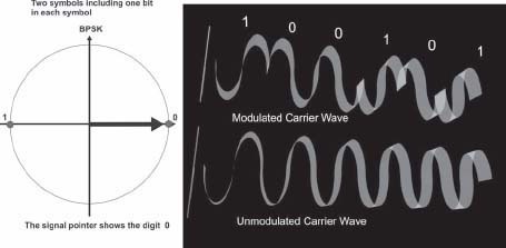
FIGURE

  4.23

BPSK is the simplest phase modulation scheme. Compared with the unmodulated wave, the modulated wave has phase jumps that do not exist in nature.

Quadrature Phase Shift Keying (QPSK)

When it comes to distribution of digital TV via satellite, a higher modulation scheme that is used, Quadrature Phase Shift Keying (QPSK).

In QPSK, there are four phase angles instead of two so each phase angle represents a combination of two digits or bits: 00, 01, 10 and 11. As a result, the radio wave may carry twice as many bits as a BPSK modulated carrier jumping around at the same speed. This means the bandwidth of a QPSK modulated carrier will only be half the bandwidth of a BPSK signal. In other words, we get twice the bitrate through a transponder when using QPSK instead of BPSK. However this benefit comes with a cost. The phase angles in a QPSK signal are closer to each other so twice the amount of transmission power or twice the size of receiving antenna will be required when moving to QPSK.

Note

The satellites of today have enough output power to make QPSK the best choice.

There are even higher modulation schemes that we will take a closer look at in the next chapter. In these modulation schemes, there are more phase angles and even several amplitude levels. Using higher modulation schemes makes it possible to get a higher bitrate throughput in the transponders but at the cost of signal quality and therefore requiring larger antennas. For this reason these schemes are only used for professional purposes when distributing via satellite.

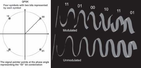
FIGURE

  4.24

Satellite distribution to the general public is based on QPSK. The modulated carrier wave has small, 90-degree jumps in phase that do not exist in the unmodulated wave.

ERROR PROTECTION AND TRANSMITTED BITRATE

In digital transmission, there are different ways of protecting the signals from disturbances. In Chapter 2, the Reed Solomon encoding technique, where 16 additional bytes were added to each packet, was described. This technique could correct up to eight errors in a packet.

This kind of error protection is used in satellite transmissions. But there is another way of securing the quality of the signal.

Forward Error Correction

By adding yet more bits to the complete signal—not on a packet-level but on a bit stream-level—the transmission quality can be secured even more. This method is called Forward Error Correction (FEC).

There are different levels of FEC. In the least ambitious level, FEC=7/8 is used. FEC=7/8 means that the extra error-protecting bits will occupy one-eighth of the total number of bits in the bit stream.

The other levels of FEC are 5/6, ¾, 2/3 or 1/2, and they require even more capacity. In the most ambitious level, FEC=1/2, half of the bits in the bit stream are required for error correction. The most common level of FEC is ¾, which is regarded as a suitable compromise between quality and use of capacity for error protections.

The bitrate calculation for a conventional 33 MHz satellite transponder may look as follows:

The useful bitrate is 38 Mbit/s. Adding 16 bytes for Reed-Solomon protection on the 188 byte packets will increase the bitrate to ((188 + 16) / 188) * 38 Mbit/s = 41.2 Mbit/s. A further use of FEC=3/4 will increase the bitrate to 41.23 * 4 / 3 = 55.0 Mbit/s. If QPSK is used to transfer this signal, the symbol rate (the speed at which the signal jumps between different phase angles) will be 27.5 MS/s (mega symbols per second).

Note

The symbol rate is one of the parameters that you will find when navigating the installation menus of a digital consumer satellite receiver trying to make a manual channel search.

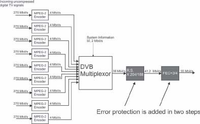
FIGURE

  4.25

In the uplink station, error protection is added in two steps before the signal is beamed towards the satellite.

DISH SIZE

The output power of a satellite is spread across an extensive area. The weaker the signal, the larger the antenna required to collect enough signal power for the LNB to produce a useable signal.

In EIRP maps showing the power radiated towards areas on the Earth's surface, it is possible to read what dish size is required at a certain location. You do not have to think a lot about decibels or dBW; instead you may regard the EIRP as a measured value. See Table 4.1.

It is of interest to notice that 6 dB corresponds to a factor of 4 when it comes to the surface of the antenna and a factor of 2 when it comes to the diameter of the antenna. In other words, if the signal strength of the satellite is increased by 6 dB, a dish with half the diameter will produce the same result, while a decrease of power by 6 dB would mean a requirement to double the diameter of the dish.

TABLE

    4.1

Suitable antenna diameters at corresponding EIRP levels in Ku-Band which is the frequency band normally used in Europe.

EIRP (dBW):	Antenna Diameter (meters):
41	1.90
42	1.69
43	1.50
44	1.34
45	1.20
46	1.07
47	0.95
48	0.85
49	0.75
50	0.67
51	0.60
52	0.53
53	0.47

Figure 4.26 shows EIRP maps with examples of some important European satellite systems. (Figures 3.28 through 3.30 on page 64 show some others.)

Using these maps with Table 4.1, you can build a quite good view about what dish size is required. More coverage maps may be found in the Web sites of the satellite operators.

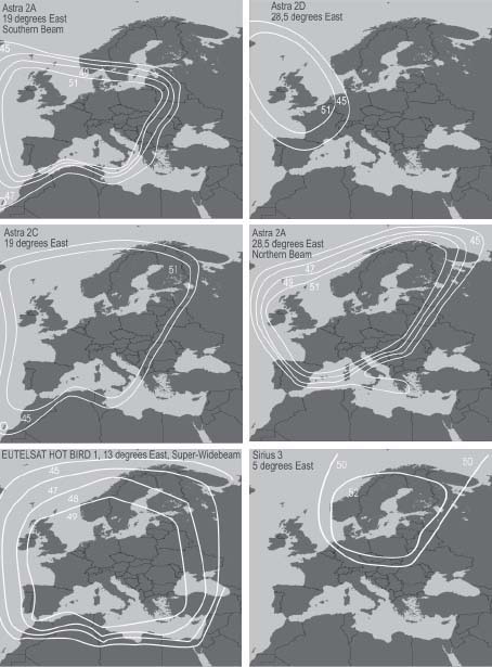
FIGURE

  4.26

By reading the EIRP in the maps and the antenna diameter in Table 4.1 identify the dish size required for reception.

MULTI-SATELLITE ANTENNAS

In the beginning of satellite TV, a separate antenna was always used for the reception of each satellite. But soon people wanted to receive signals from several orbital positions. In an ordinary home or on the balcony of an apartment, you don't want to have a dish farm. Times are since long gone when it was status to have a satellite dish.

New kinds of multi-satellite antennas have been developed. By putting more than one LNB in a parabolic dish, it is possible to get a fixed antenna to look in several directions toward different orbital positions.

A parabolic dish actually has several focal points. A signal hitting the dish along its main axis is concentrated in the main focus. This, of course, is the most efficient focal point. However, a signal hitting the dish from a slightly different angle will get concentrated at a secondary focal point. This focal point is not as efficient as the primary, but still useable to locate a second LNB. This LNB can be used to receive signals from a second orbital position.

In Table 4.2, the antenna size required for the use of a secondary focal point at different EIRP values is shown. In comparison to Table 4.1, where the LNB is located in the primary focus, a larger antenna is needed. The values in Table 4.2 are based on an example separation between the primary and the secondary orbital slot of six degrees, such as between Astra 1 at 19 degrees east and Eutelsat HOT BIRD at 13 degrees east.

In the Scandinavian countries, such antennas are used for simultaneous reception of signals from the Sirius and Thor systems that are also at a separation of six degrees.

TABLE

    4.2

Antenna Diameter Required for Secondary Focus (six degrees of separation)

EIRP (dBW):	Antenna Diameter (meters):
44	1.90
45	1.69
46	1.50
47	1.34
48	1.20
49	1.07
50	0.95
51	0.85
52	0.75
53	0.67
54	0.60
55	0.53
56	0.47

The “Two-Orbital Position” Dish

The most common multi-focus antenna is the dish covering two orbital positions. Many Europeans are interested in receiving both main positions of the Astra and Eutelsat systems at 19 and 13 degrees east respectively. Six degrees of separation is the magical figure.

There are two ways of designing a two-focus antenna. One way is letting one of the LNBs be in the main focus providing maximum efficiency for one of the positions. The second LNB is located in a way that gives six degrees of separation. Pointing the antenna towards Eutelsat, 13 degrees east, optimize the antenna for this orbital position. Letting Astra use the secondary focus will require better signals from this orbital position. This could be a good compromise, since Eutelsat HOT BIRD, having some of its transponders in a wider European beam, provides some weaker signals than Astra and therefore needs a stronger receiving position. Still, stepping up from a 60- to an 80- or 90-cm antenna will provide good reception of both orbital positions in most parts of Central Europe. However, if you are at the edge of coverage, other solutions might be better.

Another alternative is to put both LNBs in secondary focus with a distance of just three degrees from the direction that is obtained at the main focus. In this case, the dish is pointed towards a direction which is right between both orbital slots. Half of the manufacturers that make multi-focus antennas in Europe use this kind of design for the dual orbital position dish.

However, in multi focus antennas there must be a way for the receiver to switch between the LNBs. The Digital Satellite Equipment Control (DiSEqC) system was initiated by Eutelsat to solve this problem.

The idea is using the 22 kHz tone, which is also used for frequency band selection in universal LNBs, to send short telegrams to remote controlled switches that are placed in the antenna. To be able to switch between Astra and Eutelsat HOT BIRD, we would need a two-way DiSEqC switch (see Figure 4.27). Inside the switch there is a small decoder that reads the messages in the 22 kHz tone. Thus, by using smart addressing the satellite receiver can make the switch to see to that the receiver always get signals from the right LNB.

Earlier tone switches using continuous 22 kHz tones to be able to switch between LNBs cannot be used with modern digital receivers and universal LNBs, since the continuous tone is engaged in switching frequency bands. Therefore all switches need to apply to the DiSEqC standard.

The universal LNB was developed at the initiative of Astra, using a very wide frequency range, while the DiSEqC standard was an initiative of Eutelsat, which had many orbital slots. Two competing satellite systems and competing strategies have led to the invincible combination of the universal LNB and the DiSEqC-switch, providing the maximum number of channels using only one dish. In a dish for HOT BIRD and Astra, the universal LNB and the DiSEqCswitch are used in combination with each other.

FIGURE

  4.27

A DiSEqC switch is required to switch in between the LNBs.

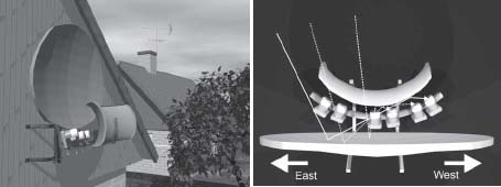
In a dish with two LNBs, the LNB that looks towards the orbital position to the west is actually located to the east of the LNB looking towards to the orbital position to the east and vice versa. In a dish for 19 degrees east and 13 degrees east, the LNB for 19 degrees east is located west of the LNB for reception from 13 degrees east. This is shown in Figure 4.28.

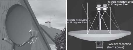
FIGURE

  4.28

Reception from 13 degrees east and 19 degrees east using one dish.

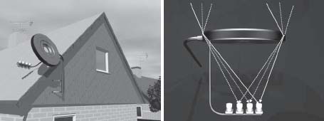
The Four-LNB Dish

It is possible to design satellite dishes that can receive signals from more than two orbital slots, such as Figure 4.29. There are DiSEqC switches with four inputs. In many countries, these are used to combine more regional satellite channels with the main European satellite orbital slots at 13 degrees east and 19 degrees east.

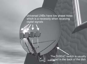
FIGURE

  4.29

Using a four-input DiSEqC switch, it is possible to combine a wide range of satellite channels in one single antenna. The size of such antennas is about one meter in diameter.

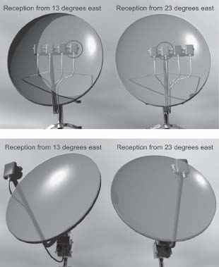
A parabolic dish with four LNBs may be configured in several different ways. In Figure 4.30, the dish is pointed towards 23 degrees east, which is the Astra 3 slot. There is also a LNB for 28 degrees east (Astra 2 and Eurobird), and one LNB for 19 degrees east (Astra 1) and finally one LNB for 13 degrees east (Eutelsat HOT BIRD).

The other combination in Figure 4.30 is popular in the Scandinavian countries. The dish is pointed towards 13 degrees east (Eutelsat HOT BIRD) and has a second LNB towards 19 degrees east (Astra 1). The third and fourth LNBs are used for reception from Sirius at 5 degrees east and Thor from 1 degrees west.

Of course other combinations are also possible.

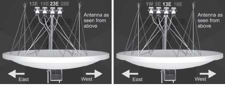
FIGURE

  4.30

A popular European configuration for four LNBs on one dish (left) and a popular Scandinavian configuration for four LNBs on one dish (right). (See color plate.)

To get a four-LNB multi-focus antenna to work, a four-way DiSEqC switch, like the one shown in Figure 4.31, is required. The DiSEqC switches are put in plastic housings for weather protection. The switches are generally put somewhere behind the antennas.

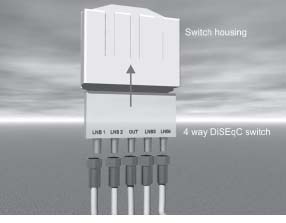
FIGURE

  4.31

A four-way DiSEqC switch in plastic housing.

More Advanced Multi-Focus Antennas

It is possible to put even more LNBs into a parabolic dish to be able to receive signals from even more orbital slots. However, there are technical limitations. One such limitation is the mechanical problem of putting LNBs too close to each other. It is hard to receive signals from orbital slots that are separated less than six degrees in ordinary parabolic antennas having a diameter of about one meter. To a certain extent, this problem may be solved using LNBs with separate, specially designed, thin feed horns (the feed horn is the front part of the LNB containing the window that receives the signal). In larger antennas, it is possible to have smaller angular distances in between the orbital slots.

Another problem is that the reception from a certain orbital slot will get less efficient as we move away from the central boresight direction of the parabolic reflector. Therefore, a conventional parabolic dish will only work properly within a limited angular distance from the boresight direction. However measures have been taken in some designs to compensate for this. One way is keeping the parabolic profile in the vertical plane of the dish while changing the horizontal profile from parabolic to a spherical profile. This makes the efficiency in reception more equal from orbital slots within a wider angular range. Figure 4.33 shows a deformed parabolic dish with a fifth LNB.

Using more than four LNBs also means leaving the standard DiSEqC applications. The DiSEqC standard is divided into different levels. At the lowest level, DiSEqC 1.0, two-way and four-way DiSEqC switches are supported. On the next level, DiSEqC 1.1, it is possible to cascade two switches, which means that up to 16 LNBs may be supported if four four-way switches are cascaded with one four-way switch. Less ambitious alternatives are possible, such as cascading two four-way switches with one two-way switch to support 8 LNBs and so on. Cascading DiSEqC switches can be tricky and it is a matter of using the right kind of DiSEqC switches programmed to use the right commands. The first and the second switch in a cascaded chain must use different DiSEqC commands. Therefore the best thing to do is to buy a complete package including a receiver supporting the DiSEqC 1.1 level and the cascaded switches that are to be used. However there is a more modern alternative.

DiSEqC Switches With More Than Four Inputs

There is a way to avoid the problems with cascaded DiSEqC switches. Cascaded switches have two major drawbacks. First the receiver has to support DiSEqC 1.1 which is not very common. Second, the cascaded switches have to respond to different DiSEqC commands; you have to have the appropriate combination of switches.

However there is an alternative. Czech manufacturer EMP-Centauri has introduced a number of switches that have a larger number of inputs (see Figure 4.32). The most amazing thing about these switches is that they can be set to respond to DiSEqC 1.0 commands as well as the DiSEqC 1.2 commands that are normally used for DiSEqC motor control. DiSEqC 1.2 allows for selection of up to 32 orbital positions using a DiSEqC motorized antenna (which is covered later in this chapter). DiSEqC 1.2 is supported by lots of digital receivers and this makes it as easy to use the multi port DiSEqC 1.2 switch as an ordinary two- or four-input DiSEqC switch.

A switch of this kind is very useful with multi focus antennas that can house a large number of LNBs as the torodial antenna.

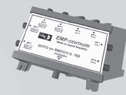
FIGURE

  4.32

The eight-input DiSEqC switch from EMP-Centauri responds to DiSEqC 1.1 as well as DiSEqC 1.2 commands.

Note

Receivers that support DiSEqC 1.2 (DiSEqC motor control) also support DiSEqC 1.0 but not necessarily DiSEqC 1.1.

In recent years, new kinds of more advanced antennas have been introduced to improve multi-focus reception. These antennas provide reception that is more equal in performance when it comes to receiving signals from different orbital slots. To obtain this, more advanced antenna techniques have been developed.

The basic idea of this kind of antennas is the torus antenna. This is based on the principle already mentioned of using a spherical profile in the horizontal plane while maintaining the parabolic profile in the vertical plane.

Using dual reflectors opens up new possibilities, both for getting a mechanical design that allows for reception from closer orbital slots as well as improving the performance of reception across the received arc. Up to about 10 LNBs may be housed in the torodial antenna from Wavefrontier. This antenna is sold under several brands in Europe and the U.S. and is available in 60- and 90-cm versions (2 and 3 feet respectively). The 90-cm dish covers an orbital range of 40 degrees allowing as little as four degrees separation between the slots.

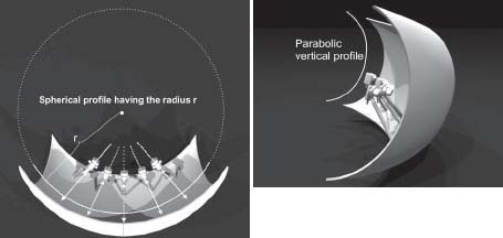
FIGURE

  4.33

The torus antenna provides better, more equal reception for multiple orbital slots.

FIG

  4.34

The “torodial” antenna is a step even further in getting an antenna with an equal performance across a wide angular range of the geostationary arc.

Other kind of less conventional antennas are the lens antennas. Lens antennas work more or less like optical lenses focusing radio waves instead of light. The performance is quite equal to the torodial antenna.

FIGURE

  4.35

The “Cybertenna” is a dielectric lens which provides a different looking satellite multi focus antenna.

INSTALLING MULTI-FOCUS ANTENNAS

When installing a multi-focus antenna with more than two LNBs, the best thing to do is to locate one LNB in the center of the dish. Then the dish will have its main boresight direction towards the satellite in the middle of the desired portion of the geostationary arc. Refer back to Figure 4.30, where we have an antenna that uses the LNB in the middle to receive signals from the orbital position of 23 degrees east. In this case, the antenna is first adjusted to optimize the Astra 3 reception using this LNB. After that, we do not have to think anymore about the direction of the reflector. Now we can concentrate on adjusting the positions of the other three LNBs one by one.

In antennas for two orbital positions, it might be a bit trickier if you go for the principle of letting the boresight of reflector point at a location in between the two orbital slots. In some smaller dishes, there is a fixed mount for the LNBs and you do not have to think about adjusting the positions of the LNBs. However this kind of arrangement means that you are stuck with a certain angular distance between the slots.

However, do not forget that the LNB to receive signals from the satellite position to the west should be located east of the LNB that is to receive signals from the orbital slot that is to the west and vice versa.

In multi-focus antennas with a large number of LNBs quite a lot of skill is required. Training makes perfection.

Motorized Antennas

Multi-focus antennas provide easy access to several orbital slots using only one antenna. However, there is always a compromise between convenience and the signal quality as well as possibilities to receive a large number of orbital slots. Multi-focus antennas are convenient since you can immediately switch between different orbital slots without having to wait for the antenna to move as is the case for the motorized antennas. But multi-focus antennas do not cover the entire visible part of the geostationary orbit. If you wish to have access to almost all visible satellites or satellites that are spread widely apart in different slots, and you are eager to receive weak signals, a motorized antenna might be the best choice.

The first motorized dishes were of the center feed (focal feed) kind, as shown in Figure 4.36, but these are not widely used today. If you are looking for very weak signals, there is still a problem in finding larger offset feed antennas. Focal feed antennas might have diameter of 1.5 to 1.8 meters or more. It is easy to know the elevation angle of such an antenna; it is at right angles to the aperture surface, as in Figure 4.36.

FIGURE

  4.36

In a symmetrical focal feed antenna, the angle of elevation is at right angles with the aperture of the antenna as is shown in this picture. The actuator, the linear motor that makes the antenna move, is on the back of the dish.

We will now take a closer look at the choice between the comfortable multifocus antenna and the more complicated but more flexible motorized dish.

A multi-focus antenna allows for instant switching between TV channels that are transmitted from different orbital slots. When choosing a channel, the satellite receiver immediately sends the right control signals to the antenna. This include the correct DiSEqC commands to the switch system, the continuous 22 kHz tone if the upper part of the frequency range is required, and the correct supply voltage to the universal LNB depending on what polarization is to be received. However, the multi-focus antenna can not provide you with optimum signal quality on all slots. The LNBs that are placed in the secondary focal points can not use the entire surface of the dish with full efficiency.

In a motorized antenna, the complete surface of the dish is always used, and antenna can be turned much farther east and west than the angular range of a multi-focus dish. You will also be able to reach orbital slots that are between those you could access with a multi-focus antenna. There are no restrictions to how close to each other the orbital slots might be when using a moveable antenna.

For practical reasons, it may still be impossible to reach the orbital slots that are extremely close to the horizon in either direction even if you have a motorized antenna. In the antenna shown in Figure 4.36, the mechanical restrictions in the mount of the antenna and the length of the actuator limit the range of the adjustment. The actuator is the linear motor that moves the antenna. In an antenna with an actuator, you select the part of the geostationary arc you wish to use by choosing at which side of the mount the actuator is situated and where the actuator is attached (there are usually a number of holes to choose from).

The drawback of using a motorized dish is that you will have to wait for the dish to move between the slots. As a consequence, the channel lists of your satellite receiver might not be arranged as you would have preferred. The order of the channels will probably follow the orbital positions rather than your taste. This is because it is not fun to zap between channels in different orbital locations when you have to wait for the dish to move. It could take 10 seconds or more to move from one slot to another. When you're waiting for a new channel selection, 10 seconds tends to feel like a long time.

As a conclusion multi-focus antennas are best suited for everyday viewing where simplicity comes ahead of technical flexibility and optimum performance. However for the technically interested person a motorized dish has more to give.

FIGURE

  4.37

Comparison between the efficiency in the use of the receiving antenna aperture for the multi-focus versus the motorized receiving antenna. (See color plate.)

DiSEqC-Controlled Motorized Antennas

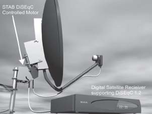
The large motorized dishes, as you can see in Figure 4.36, to a large extent disappeared from the market by the mid 1990s. At that time, many believed that the motorized antenna story had ended, but turned out not to be the case. An Italian family company, STAB, developed a very small and compact motor that uses the DiSEqC 1.2 protocol commands. The motor really both looks like and works like a part of the antenna mount (see Figure 4.38). Since it is DiSEqCcontrolled, the motor uses the existing cable between the satellite receiver and the antenna, as well as the supply voltage for the LNB. No separate control unit or power supply is needed.

For many years the manufacturers of satellite receivers had problems in following the DiSEqC 1.2 standard. This meant that STAB motors, as well as competing motors, required proprietary software in the DiSEqC motors. These days, the situation is more stable and you can buy your satellite receiver and DiSEqC controlled antenna motor from different sources and still get it to work.

FIGURE

  4.38

The STAB motor looks like an integrated part of the dish mount and it does not require any extra cabling or power supplies.

It would have been possible to design a motorized dish where the antenna could be moved around two axels—one for elevation and the other for the azimuth angle adjustment. Such antennas exist in uplink stations. But for consumer use, there is a lot to be gained from designing a mechanical mount where the antenna only has to be turned around one axle. Using a very cleverly designed mount makes this possible.

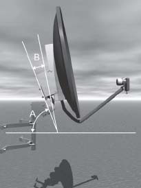
The principle of doing this is called polar mount and is based on having the dish mounted on an axle leaning at an angle A in relation to the horizontal plane and letting the reflector lean in relation to this axle with an angle B (the tilt angle). The angles are shown in Figure 4.39. The value of each angle depends on the location of the dish.

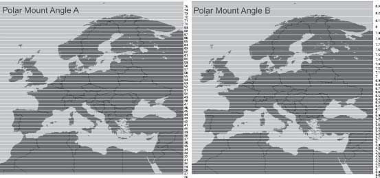
To read the angles A and B from Figures 4.40 is easy. To adjust the mount for optimum performance across the geostationary orbit might be harder and will probably takes some time. The manufacturers of antennas suggest different methods and they have their own tricks. However, in my experience, the best way to go is to start adjusting the vertical angles A and B.

It is very important that the antenna mount (STAB motor) is attached to a tube that is absolutely vertical. This may be checked with a level or weighted string.

FIGURE

  4.39

The main angles in a polar mount.

FIGURE

  4.40

The A (leaning axle angle) and B (tilt angle) of a polar mount. (The corresponding angles for North America are shown on page 307).

First adjust angle A. This might be done using a protractor and a weighted string. There are also other instruments from the construction business that might do the job. Then, adjust the B angle. In some cases there is a scale on the mount/DiSEqC motor that could be helpful when doing this.

The really hard thing is to get the north to south direction right. If you are lucky you happen to be on the same longitude as a satellite. I am lucky enough to live exactly on the longitude 13 degrees east which means Eutelsat HOT BIRD is directly south of me. If you have a satellite straight to the south you can easily use this to get the north-south line exactly right. Turn the motor so that the antenna is right in the middle position, with maximum elevation. Then just turn the complete mount to get the maximum signal strength from the satellite located directly south.

However if you are not that lucky not having any satellite straight south you have to do it in another way. Choose a suitable satellite as reference satellite. From the maps showing the elevation and azimuth curves, read the elevation angle for that satellite. Then measure the elevation angle of your antenna using a weighted string and a protractor. Now turn the dish using the motor to the east or to the west until the elevation angle of that satellite is achieved. If the satellite is on a longitude to the west of your position you should turn the dish to the west. If the selected satellite is to the east then turn the antenna to the east. Check carefully that the right elevation angle really is achieved. Now, adjust azimuth angle of the complete mount of the antenna (without turning the motor) until you receive an optimal signal from the satellite you selected.

It is not suitable to use a satellite that is in the middle of the orbit. It is better to use a satellite further out since the elevation angle falls steeper farther away from the direction towards the south. This makes the adjustments more sensitive, giving you a better accuracy when adjusting the north to south alignment of the antenna mount.

Still it is not easy finding your way through the satellite jungle. To make it easier to install the system, there might be preset channels in the memory which act as reference channels or thumbprints for each satellite.

If you are having problems in finding certain channels or certain satellites there are sites on the Internet with accurate information on the subject. One such site is www.lyngsat.com, which contains detailed information and useful links for almost all satellite channels in the world.

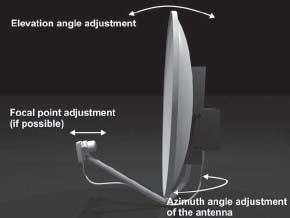
OPTIMIZING PARABOLIC ANTENNAS

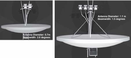
Until now, we have concentrated on how to find the approximate alignment of an antenna for satellite reception. The main problem however is that a satellite reception antenna works at very high frequencies. As a result, the antenna requires a very high degree of pointing accuracy. The pointing accuracy required is considerably higher than is the case for a terrestrial TV aerial. The angular range, where it is sensitive to incoming signals, the 3 dB beamwidth (the angular range within which the incoming signal is at least half of the maximum on boresight input power) is very narrow. A 70-centimeter dish has a beamwidth of just 2.6 degrees. In a somewhat larger dish (1.1 meters) the beamwidth is about 1.5 degrees. In these cases, you need to be able to measure the strength of the signal when making the alignment of the antenna. Someone informing you about whether or not there is an image on the TV screen is not good enough.

FIGURE

  4.41

A 70-centimeter dish has a 2.6 degree beamwidth while a 1.1 meter antenna has a beamwidth of about 1.5 degrees.

Finding the Optimum Focal Point

In this chapter we have anticipated that there is only one way to attach the LNB in the antenna. There are antennas with a fixed attachment, leaving no adjustment to the installer. However in many antennas, there are possibilities to adjust the position and orientation of the LNB. As we have learned from the multi-focus antennas, the receiving beam direction will change as we move the LNB. Therefore, adjusting an LNB into what we believe is the main focus of a parabolic dish can be tricky. If we move the LNB, the direction of sensitivity also moves. Therefore the search for the optimum focus is an iterative process moving the LNB and realigning the dish several times before the goal is reached (see Figure 4.42).

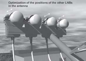
In a multi-focus antenna, it is only the LNB at the central, main focus that may be adjusted this way. As soon as this LNB works in an optimum way, you should not touch the direction of the antenna any more. The other LNBs must be adjusted by their individual positions within the antenna itself (see Figure 4.43).

FIGURE

  4.42

Iterative adjustment to get the LNB at the optimum focal point of the reflector.

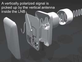
In the previous chapter, we saw that the satellites transmit both horizontal and vertically polarized signals. This makes it possible to reuse the complete frequency range and double the available bandwidth. Therefore it is necessary to orient the LNB in such a way that the small antennas inside are oriented to coincide with the orientation of the transmitted signals from the satellite (see Figure 4.44).

FIGURE

  4.43

As soon as the LNB in the centre position of the antenna works at its optimum the orientation of the reflector should not be further touched. Instead it is the individual position inside the antenna of the other LNBs that need to be adjusted.

If the orientation of the LNB is wrong, the signals from both polarizations will get mixed and the reception will not work properly. If this happens, the horizontally and vertically polarized signals will interfere with each other.

Normally the signals from the satellite are oriented in such a way that the horizontally polarized waves coincide with the equatorial plane of the Earth. The vertically polarized signals are at right angles with the equatorial plane.

A satellite that is located on the same longitude (directly south) as the reception site will transmit its horizontally polarized signals parallel with the horizon. And the vertical signals will come in polarized at right angles to the horizon. For satellites located at other slots further to the east or the west, the polarization planes will lean and be in parallel with or at right angles to the geostationary arc at it is seen from the ground in Figure 4.2.

FIGURE

  4.44

The internal antennas must align with the incoming signals.

Measuring Digital Satellite Signals

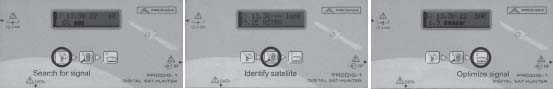
The adjustment of the polarization angle is probably the most difficult part when installing a satellite dish. High-quality measurement instruments are needed to get it all right. The alignment process for a satellite dish follows in three steps: find the signal from the satellite, identify the satellite so that you know what you are receiving, then optimize the antenna for the best reception.

Promax Prodig-1

A good example of a professional measurement instrument for this purpose is the Spanish Promax Prodig-1. Prodig-1 is a pretty small instrument that is used outside at the antenna. It has a built in battery so you do not have to rely on power from the satellite receiver.

There are three buttons and a display on the unit (see Figure 4.45). Pressing the first button triggers the search mode when the instrument just looks for signals using an indication bar on the display and an audio signal with a frequency that gets higher as a higher signal level is achieved. Pressing the second button makes the instrument to go into “fingerprint” mode where you can check different preset transponders to check that you have found the right satellite. The instrument includes half a digital satellite receiver—it is able to demodulate and demultiplex the transport stream. You can add or rearrange the presets to fit your needs as new satellites come along.

Pressing the final button switches the instrument to bit error measurement mode. The quality of the received signal can be measured by checking errors among known bits that belong to the frame structure of the DVB transport stream. By doing this, you can adjust the polarization isolation of the LNB very accurately. It is also possible to adjust for all other errors and problems that may be related to the antenna.

The Prodig-1 is very practical since you can wear on a belt, leaving both hands free. The LCD display is easy to watch even in bright sunlight.

Instruments of this kind cost a few hundred Euros or dollars but the investment will pay off if you install a lot of antennas. The reason for the cost is partly that the instrument contains almost a complete digital receiver. It also comes with software that enables you to put in new presets by connecting a computer.

FIGURE

  4.45

Promax Prodig-1 is a small and handy instrument to detect, identify and optimize the reception of a digital satellite signal.

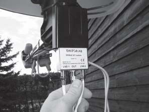
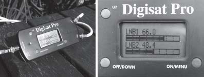
Emitor Digitsat PRO

A more semi-professional instrument is the Emitor Digisat PRO (sold in the United States as Accutrac 22 Pro). This instrument has a very special feature. It has two inputs, so it is possible to monitor the signal level from two LNBs simultaneously. This makes the instrument very interesting when installing two LNB multi-focus antennas. However, it is only possible to measure signal level; it does not measure signal quality. The signal level is not only a product of the strength of the satellite signal but also the length of cable between the LNB and the instrument, the gain of the LNB and a few other parameters. Like many other instruments of this kind, the Digisat PRO is powered by the supply voltage from the satellite receiver.

The Digisat Pro goes at about 100 euros ($130 U.S.).

FIGURE

  4.46

Digisat Pro from Emitor is a small instrument that can measure the signal level from two LNBs simultaneously.

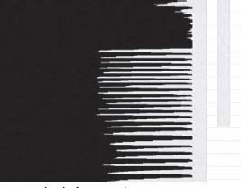
Spectrum Displays

Technical radio enthusiasts have long wished for a spectrum analyzer, for a graphical display of what a larger or smaller portion of the radio spectrum looks like. But spectrum analyzers are expensive.

Emitor has produced a small,relatively inexpensive device, the Spectralook, which you connect to your TV set. The satellite dish is connected to the device using a splitter (for simultaneous reception with an ordinary satellite receiver). On your screen you can now see all signals that leave the satellite dish in the frequency range 950 to 2150 MHz (see Figure 4.47). Each spike in the spectrum corresponds to a transponder; the longer the spike, the stronger the signal from that particular transponder.

It is not possible to use the Spectralook to make any actual measurements, but still you get a very useful graphical display showing the signals being received. This instrument is very useful if you have a motorized antenna and you are on the hunt for “new and unknown” signals. When the antenna passes by a satellite you will immediately see its signals on your screen and you can then investigate the signals in detail using your digital satellite receiver. This is an instrument good for finding the needle in the haystack.

FIGURE

  4.47

Spectralook from Emitor converts your TV set to a spectrum analyzer. The spectrum is symbolized vertically where each spike corresponds to a transponder.

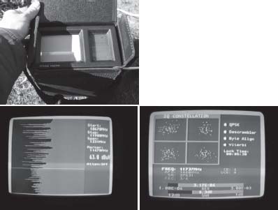
Emitor also makes the Satlook Digital (also sold in the U.S. under the same name), a more professional instrument that includes a spectrum display. This very advanced instrument not only produces an image of the spectrum but also performs actual carrier-to-noise measurements based on bit error rate measurements and calculations. A fascinating feature is the constellation diagram display, where you can see samples of the phase angle and amplitude registrations on actual signals—an actual phase diagram of the QPSK signal as is shown in Figure 4.48.

Another great feature of the Satlook Digital is that you can transfer all measured data to an external computer for documentation purposes. This is not an instrument for consumers but could be a goldmine for professional installers and satellite enthusiasts.

FIGURE

  4.48

Satlook Digital from Emitor is both a simple spectrum analyzer and a measurement instrument that decide the signal quality from bit error measurements. It can also display the constellation diagram of a QPSK modulated signal.

Recommendations for Consumers

But what should ordinary consumers do if they want to install the dish themselves? To do the installation without some kind of instrument is not easy. One option is to try to borrow a simple “Satfinder” from the shop where you buy the receiving equipment. Such instruments are not that expensive to buy either. The cheapest instruments in the market are the “Satbeepers” (see Figure 4.49). This is a small device that is connected to the LNB and gets its supply voltage from the satellite receiver. There is a small earphone that indicates the signal strength by a beep. The frequency of the beep corresponds to the strength of the signal. Satbeepers sell at a less than 20 euros ($25 U.S.).

Stepping up to the next instrument will cost 40 to 50 euros ($50 to $65 U.S.) and will provide you with a visual indication of the incoming signal either as meter with a needle on a scale or an LCD indication bar.

The problem in using these inexpensive instruments is that they do not provide you with any identification of which satellite you receive and you are not able to measure the signal quality. The latter means that you will not be able to adjust the polarization because you have to be able to measure the bit error rate in some way.

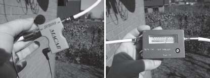
FIGURE

  4.49

Satbeepers and Satfinders are the smallest and cheapest among the large number of instruments that are available in the market.

To do this you have to step up to the professional instruments that generally go at between 500 to 1000 euros ($640 to $1,280 U.S.). All these instruments have in common that they are used outside close to the antenna so you can adjust the dish as you are measuring the signal. A spectrum analyzer is the most professional way to go, but I must say that an instrument like the Promax Prodig-1 is very appropriate to get the job done even though it is not as fancy as a spectrum analyzer.

There is another very cheap way of measuring the signal quality. Your digital satellite receiver is really an advanced measuring instrument. It has the ability to measure the signal strength as well as the signal quality. In many cases, there is a menu that contains measuring bars that show these two parameters. The receiver can measure the bit error rate by counting errors among known bits that are a part of the DVB framing structure. If you see that the signal quality is at a high level you probably have the polarization adjustment done correctly.

For obvious reasons, most dishes are installed when the weather is good. However many times when you watch TV, it is raining. And when it is raining, you may get problems with your satellite signal since that is when the microwave signals are attenuated in the atmosphere. It is quite important to check the signal quality as soon as the installation is done.

In the analog days, you could see from the presence or absence of noise the margins in your receiving system. But digital signals don't provide that. As soon there is a picture it is 100% okay. So, if you have a bad margin you might lose your picture completely when it starts to rain.

Therefore the quality measurement menu is the only way to know the margins. And if it should happen that the signal disappears or get disturbed during a heavy rain shower, it may also be interesting to check the signal quality for future reference. Then you know at what quality level you will lose the picture.

However it is essential to get to know which of the measurement bars in the menu system that measures the signal quality (see Figure 4.50). In some cases, there might be a bar only reporting the signal level. This is not as interesting as the quality since the signal strength depends on several other things, such as the length of the cable in between the LNB and the receiver.

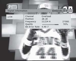
FIGURE

  4.50

The menu system of the satellite receiver may contain many useful things. One of the most useful, but also one of the least known, is the built in signal quality metering system. In this receiver from Digitality, the quality is both represented as a bar and in figures providing the bit error rate (BER).

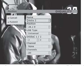
When aligning a satellite dish, it is essential to know that you have found the right satellite. In many cases the receiver is pre-programmed with some known channels on each satellite position. But you always have to start off telling the receiver what the antenna system looks like. Information such as how many LNBs are attached to the receiver and at what inputs of the DiSEqC switch these are connected is necessary for the receiver to find the channels. This is done with the antenna configuration menu in figure 4.51. As soon as this is done, the receiver will be able to search for channels in each slot by itself, provided, of course, that the antenna is properly aligned.

An alternative to automatic channel search is to search for certain channels manually. This may be done by entering the frequency, polarization, symbol rate and FEC of a certain transponder. On top of this you may specify what you are looking for down on service level by entering PIDs. However, manual search is an alternative only if you know exactly what you are looking for and don't want to update an entire orbital slot, which might take some time.

In most cases the automatic channel search preferable. You just select the orbital slot you'd like to update and then let the receiver do the job (see Figure 4.52). The channels are picked up in an automatically generated list. If you have a dish that includes the large European orbital slots, it may take a while to search it all. But afterwards you might have between 2,000 and 3,000 channels in the list. A lot of channels may be unavailable since they are encrypted and only available in other countries. But still there are several hundreds of channels from all corners of Europe available.

FIGURE

  4.51

In the antenna installation menu you tell the receiver on which LNB to find a certain orbital slot.

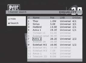
FIGURE

  4.52

You do not have to search for the satellite TV channels by yourself. Just pick the orbital slot you like and let the receiver do the job.

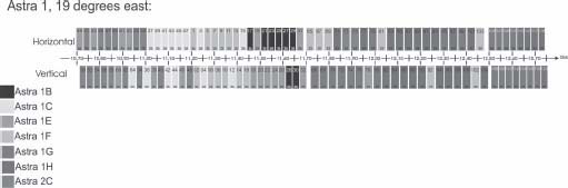
Today each orbital slot may contain an almost uncountable number of radio and TV channels. In the 1990s it was still possible to zap between all available satellite TV channels in one night. Perhaps it still is. But almost nobody does that anymore. Figures 4.53 and 4.54 contain the transponder plan for Astra 1 (19 degrees east) and Eutelsat HOT BIRD (13 degrees east). Every transponder may contain up to about 10 TV channels or a very large number of radio channels.

FIGURE

  4.53

The frequency plan for Astra at 19 degrees east. (See color plate.)

FIGURE

  4.54

The frequency plan for Eutelsat HOT BIRD at 13 degrees east. (See color plate.)

Coaxial Connectors

Finally there is a small thing that always needs to be done when installing a satellite dish. You have to bring the coaxial cable from the dish into your house. In order to pull the cable through a hole in the wall, you cannot have a connector on it. For this reason, you will have to put the connector on to the cable by yourself (once that end is in the house), even in a world of ready made cables.

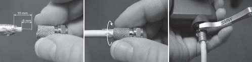
The connectors used for the LNB to the receiver cabling when it comes to satellite TV are the F connectors. They come in many different kinds, but the simplest one to use is the “Twist-On” F-type connector. Figure 4.55 shows how to put such a connector on to a coaxial cable. Remember to use the right size of connector to the dimension of cable that you use. If you have a multi-focus antenna you should take advantage in using ready made cables to connect the LNBs and the DiSEqC switch.

An important issue is weather protection. Nowadays, weather protection of the connector that is attached to the LNB is achieved by using a rubber hose that is attached to the LNB itself and that covers the F connector completely. An old alternative was to use vulcanizing tape that kept the connector moisture-free for a long period of time. Another place where weather protection is necessary is at the connectors for the DiSEqC switch. Nowadays the manufacturers have developed clever solutions for this.

FIGURE

  4.55

The “Twist-On” F type connector is perhaps not the most professional kind of F type connector but it is no doubt the most common one.