At the core of the Path Finding system is an algorithm that calculates the shortest navigable path between two points on NavMesh. Dijkstra's algorithm is named after the computer scientist Edsger Dijstkra, who originally created it in 1956 and later published it in 1959 to find the shortest paths between two points. There are a few path finding algorithms worth mentioning, but the most commonly used in gaming is a variant of Dijkstra's algorithm. The variant is called the A* algorithm. A* works by having a list of traversable points. Then, from the start position, we want to search for the shortest path in each available direction. We can determine this by heuristic values. These values will tell us how much it costs to traverse to the next point based on some predefined rules. In A*, we traverse from a point to another point to reduce the exploration cost. The big difference between the two algorithms is the fact in A* that you have a heuristic value, which affects your pathing decisions. Heuristic values are obstacles to the predictive cost to travel to the next possible point. When the path is generated, we want the lowest heuristic value. So this means that by setting the heuristic values to 0, the algorithm is the same as Dijkstra's. Dijkstra's algorithm scans more nodes, usually making it less efficient because it doesn't predict the cost of traversing paths.

Let's take the following grid as an example:

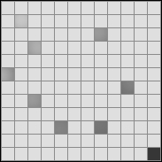
Dijkstra's algorithm takes every available point into account. So, in this example, we'll start from the upper-left corner and try to get to the lower-right corner, and all the adjacent nodes are considered to be connected and can be traversed from each other. Perform the following steps:

This can take a lot of steps, and that's the reason for which we adapted heuristics in A*. Instead of searching each node, we will continue from the shortest current path to the goal.

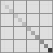
An example with A* is represented in the following grid. The algorithm will start from the first node (in the upper-left corner) and then scan the neighboring nodes to calculate the movement cost. The node at which the cost is the least is selected, and the nodes that are not selected are put on the list of the scanned nodes. This avoids us having to go to these nodes again for this query:

From step 1, the neighbouring nodes are scanned and checked for heuristic values or path cost to determine the next optimal step. What results is a direct path (if unobstructed).

There are other algorithms available, but A* is easy to implement and isn't resource-heavy, so it is commonly implemented in gaming engines as a way of creating paths between two points on a grid.