
Computers operate in time and space. In this metaphor, instructions represent time and memory is space.
In the real world, factories optimize their space. Parts must flow from one place to another for maximum efficiency. If distances are too great, time becomes a factor. If the space is not laid out well, workers cannot complete their tasks efficiently.
Inside CPUs, transistors switch ever faster. However, the speed of light imposes hard limits. A chip—a single computational unit—cannot be the size of a room. It must fit into a small footprint. Electrons have to transfer charges from one part of the machine to another for work to be done, and while transistors are orders of magnitude faster than they were a few decades ago, electricity travels at the same speed now that it did at the beginning of time.
Similarly, as on-die memory sizes, such as L1 and L2 caches, increase, we are bound by the amount of memory we can access in a fixed time period. Hundreds of instructions can be processed in the time it takes a cache line to be fetched from main memory. Caches help, but they are expensive and limited in size by physical and financial constraints.
Herb Sutter suggests that CPU clock speed increases have outpaced memory speed increases by 150% since the early 80s. Rico Mariani, a software architect at Microsoft, likened the modern processor to driving a sports car in Manhattan (Sutter, 2007). Optimizing the CPU is like driving a car: You can spend your time optimizing the car or removing the stoplights. In this context, stoplights are cache misses, and they affect performance more than you would expect. The faster your CPU, the better your code needs to be about reducing cache misses; otherwise, your sports car is idling at stoplights instead of cruising down straightaways.
Naturally, optimizing memory at a fine level is going to be very hardware-specific. Different memory topologies and processors have different requirements. If you tune an algorithm too far for a specific processor, you might find that you’re hitting a performance cliff on another processor. Because of this, we will spend our time focusing on general techniques that give better performance in all cases. As always, we will measure our performance at every step so that we avoid performance pitfalls.
This chapter will also guide you toward a more specific understanding of memory performance. A program is not just “memory” bound; there are always underlying problems, such as bus bandwidth or capacity, and various solutions, such as access patterns or alignments.
The problems discussed in this chapter do not really end with data. Instructions, after all, are represented by data. The CPU has to fetch them from memory just like everything else, and in some situations, this can become a factor in performance.
Memory access is invisible in most cases. Unless you are looking at assembly, the means of memory access are pretty much invisible. You might be accessing a register, the stack, the heap, or memory space mapped to a device on the other end of a bus. The data might be cached in L1, L2, or L3 cache. It might be aligned or not.
Memory access is invisible until it becomes a problem. Because of this, it’s easy to overlook. If an algorithm is slow, is it because it is using memory in a slow way, or because it is doing a lot of computation? Sometimes, this can lead to counterintuitive situations. For instance, a binary search is faster from a big O perspective, but it may have bad memory access characteristics because it is jumping around randomly. A linear search may be much faster if it can take advantage of hardware pre-fetching, even though it is doing more work. A lot of the time, the size of the dataset is the tipping point in these trade-offs.
The best tool for finding memory-related performance analysis is an instruction-level sampling profiler like gprof or VTune. If memory is a bottleneck, then you will see a lot of time being spent on seemingly innocuous memory load instructions. Profilers that read hardware counters (like VTune or Code Analyst, which both work on AMD and Intel chips) are also useful because they can tell you which regions of your code are causing lots of memory stalls or cache misses.
If you don’t have special tools, hope is not lost (but you may have to do more work). If you have basic timing capabilities, it’s easy to guess-and-check to find hotspots in execution. From there, you can do visual inspection (or experimentation if you have a benchmark) to see if it’s memory access that’s hurting you. For instance, you might temporarily change a loop to do the same amount of work but only over the first item in an array. That removes cache misses as a potential source of performance loss.
First things first—you have to determine if the application is CPU bound. There’s no ROI optimizing the CPU when another resource is the bottleneck! We’ve covered how to do this already in Chapter 5’s discussions on CPU-bound applications.
After you’ve identified the CPU as a bottleneck, the next step is to look for cache misses. CPUs have counters to measure this, so you have to find a tool to access them; otherwise, you will spend your time looking for what you think are cache misses. Learning the patterns that cause cache misses is the main topic of the remainder of this chapter.
Using VTune to Find Cache Misses
VTune sampling provides a useful means for detecting performance issues caused by cache misses on CPU-bound applications. This example uses the Performance Test Harness test: “memory/traverse/randomStatic.”
First, open the Advanced Activity Configuration (one way is to right-click the activity) and add the following VTune Event Ratios to the sampling:
L1 Data Cache Miss Rate
L2 Data Cache Miss Rate
If the highest function hotspot for time is also the highest hotspot for data cache misses, then it’s time to use the tips in this chapter to get the best ROI.
In Figure 6.1, the yellow bar represents the time spent inside of a function. The biggest opportunity for performance increase is the initStatic function; therefore, it’s probably a better idea to optimize or remove that function before optimizing for L1 (light red) and L2 (dark blue) cache misses.

Figure 6.1. Comparing time to cache misses is important when considering the performance impact of cache misses.
Always consider time when optimizing for memory. UtilCacheRandomizer::scrambleCache has more cache misses; however, the net effect on performance is not as bad as the StaticMemoryPerformanceTest:test function, which consumes more time.
Physical constraints make it difficult for hardware manufacturers to decrease memory latency. Instead of trying to break the speed of light, manufacturers focus on hiding latency by using caches and predictive techniques like pre-fetching.
The best tactics for optimizing memory usage involve leveraging the cache:
Reducing memory footprints at compile and runtime
Writing algorithms that reduce memory traversal/fetching
Increasing cache hits through spatial locality, proper stride, and correct alignment
Increasing temporal coherence
Utilizing pre-fetching
Avoiding worst-case access patterns that break caching
Two of these tactics are simple, and we’ll cover them immediately. The others are more involved, and the following sections will address them. Fundamentally, all of them are about using the hardware in the most efficient manner.
Reducing the memory footprint of your application is the same as getting a bigger cache. If you can access 16 bytes per item instead of 64, you are able to fit four times as many items in the same size cache. Consider using bit fields, small data types, and in general, be careful about what you add to your program. It is true that today’s machines have a lot of system memory, but caches are still on the order of several megabytes or less.
Reducing memory traversal or fetching relates to the importance of application optimizations. The fastest memory is the memory you don’t access; however, the price of L2 cache misses, in the magnitude of hundreds of cycles, is so high in comparison to cache hits, that a developer should be aware of the trade-off between naïve algorithms that traverse memory with few cache misses and algorithms that fetch memory less often and cause many cache misses.
CPUs may perform automatic hardware pre-fetching in an attempt to hide latency by recognizing memory access patterns and getting “ahead” of the executing program’s memory needs.
This is generally a win. It allows the hardware to deal with otherwise naïve algorithms. It hides the latency in the system and requires no difficulty to maintain pre-fetching logic from developers or compilers. As always, you should measure to make sure that hardware pre-fetching is helping you. There are scenarios where it can hurt rather than help.
Hardware pre-fetching does not typically help with small arrays. Hardware pre-fetching requires several cache line misses to occur before it begins. Therefore, an array that is only a few cache lines in size, on the order of 128 bytes (Intel Software Network, 2008), will cause useless pre-fetching, which consumes bandwidth unnecessarily.
The alternative to automatic hardware pre-fetching is software pre-fetching, a topic we will discuss later in this chapter. In general, the hardware pre-fetch is preferable to the software pre-fetch, since hardware pre-fetch decouples your code from the pre-fetching implementation. However, you may encounter hardware that does not implement hardware pre-fetch, or you may encounter one of those rare situations where software pre-fetching truly is a win.
But choosing the “optimal access pattern” is easier said than done. The only way to find the best patterns and more importantly see how much of a difference there is between different patterns is to test. As part of the performance tests that come with this book, we have implemented several different traversal patterns and compared their performance.
The code shown here in the text is simplified to make its operation very clear. In practice, the compiler will optimize them to nothing. Review the memory/traverse section of the test suite in order to see the details of our implementation.
We will discuss each pattern and then compare its performance.
The first access pattern we will discuss is a linear access forward through an array of integers:
for( int i=0;i<numData;i++ )
{
      memArray[i];
}
Next, let’s consider the same loop, but instead of stepping through code from front to back, let’s move back to front. We will call this linear access backward through memory.
for( int i= numData-1;i>=0;i–– )
{
      memArray[i];
}
Next, let’s step through memory using regular strides. This sort of traversal occurs when you step through a list of structures and access only one member. We will call this access pattern periodic access through memory:
struct vertex
{

     float m_Pos[3];
     float m_Norm[3];
     float m_TexCoords[2];
};

for( int i=0;i=numData;i++ )
{
      vertexArray[i].m_Pos;
}
Finally, the last access pattern we will discuss is random access. This one is important because it typifies most complex data structures. For instance, a linked list, a tree, a trie, or a hash table will all exhibit fairly random access patterns from the perspective of the hardware. The code for random access is:
float gSum = 0;//global memory

void Test()
{
      for( int i=0;i=numData;i++ )
      {
         gSum+=vertexArray[RandI()]; //actual code uses a pre-
      }                              //randomized array instead
                                     //of RandI() due to
                                     //latency
}
Now, you can see the results of our tests in Figure 6.2:
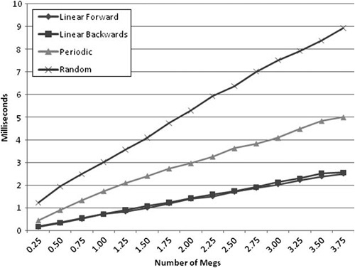
Figure 6.2. Linear forward and linear backward access patterns have nearly identical performance when stepping through 1 to 4 megabytes of global memory. Our workload is performing floating-point addition on the stored 32-bit values.
Let’s discuss these results. Notice that the linear access forward and linear access backward times are nearly the same. In fact, it’s difficult to tell that there are two lines. The slope is also low relative to the other approaches, which is indicative that hardware pre-fetching is reducing the cost of traversing the memory.
Now look at the random access line. The slope is much worse than the linear lines—pre-fetching, if it is occurring, has less benefit. The difference is large at every dataset size. Finally, the periodic access falls between the linear and random patterns. Depending on the stride size, different results will occur. As we increase stride size, we see the performance move closer to that depicted with the random line (and in some unique cases, periodic access can have worse performance than random—more on this later in the section, “Fix Critical Stride Issues”).
Allocating memory in big chunks for linear traversal can be more difficult, but as the previous chart shows, the returns are significant. Graphics APIs do a good job of forcing you to give them memory in big buffers through objects like vertex buffers.
However, you will not always be working with linear arrays of data. It may not be possible to design for linear access in every situation. Allocating and freeing may become too costly if you maintain a linear array. Or the data may need to be traversed in a specific order. You have to weigh the trade-offs when you implement or choose data structures.
There are solutions that lie between fixed allocation and a dynamic allocation; using the strategy of a dynamic array provides more flexibility with cache advantages of linear memory. Instead of allocating and deallocating objects one at a time, use blocks to batch the overhead effectively. When adding objects to a dynamic array, allocate large blocks by a “bucket size.” This bucket size can change dynamically as well. Many implementations of dynamic arrays grow the bucket size as the array count grows. A bucket size of 5 may be appropriate for an array that will never grow over 50. An array that is the size of 1,000 would probably benefit from a bucket size of 100.
For bulk data processing, the chart shows the benefits of linear access. However, there are some trade-offs at work that you should be aware of. In some cases, linear access isn’t always best.
The more common case is when nonlinear traversal lets you reduce your working set significantly—the random access times are below the linear access times when the working set is about an eighth of the size. A tree structure can easily give you this kind of reduction. You will want to measure before deciding on one option over another.
The other situation is less obvious. If you have a lot of computation to do on each item, then you can “hide” the cost of out of order accesses via pre-fetching. Of course, this requires you to think through your access pattern carefully, and you will need to be able to calculate the pre-fetch location before the previous computation ends. For more info on pre-fetching, see “SSE Loads and Pre-Fetches” near the end of this chapter.
While the CPU is crunching away at the work of each memory location, the memory system can be fetching data in anticipation of its use. When you access memory linearly forward or linearly backward, the hardware pre-fetching is at its best and the cache is used most efficiently.
Is random access always slower? It depends on the scale. Cache lines act to even out small-scale randomness. For instance, if you have a small struct and access its members out of order, you may not notice a difference in performance. If the struct fits in a cache line and is aligned, then the order won’t matter at all because accessing one member has the same cost as any other. As the scale of randomness varies, for instance with larger structs, then the effects are more pronounced.
How Random Is Random?
We have implemented a test to explore randomness confined to a stride size. This source for this test is available in the Performance Test Harness: “memory/traverse/linearLT512byteRandomStatic.” The results are shown in Figure 6.3.
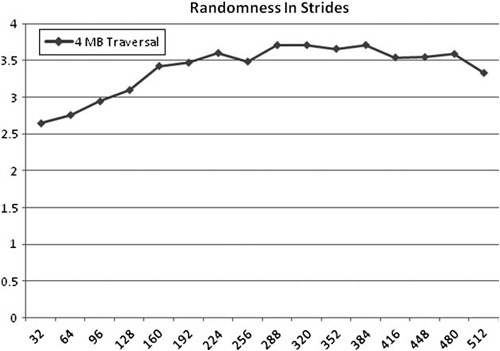
Figure 6.3. Randomness in fine granularity (from 0 to 512 bytes granularity) yields the best performance when randomness strides are very small.
Each data point represents traversal through four megabytes, with the stride of random access getting larger at every point. This performance test is similar to stepping through an array of structures and accessing each current structure’s member in a random order.
So far, we have only discussed automatic hardware pre-fetching’s impact on accessing a single stream of memory. Most CPUs can actually support multiple streams. The number of effective streams is difficult to generalize. It depends on the number of active processes, the specific chip, operating system behavior, and so forth.
The Intel documentation suggests that the number of concurrent streams in Intel processors differs from processor to processor but is in the range from 8 to 16 (Intel, 2008). The best practice is to measure it—which we’ve done—and design your application to rely on a minimum of memory access. Figure 6.4 shows our results.
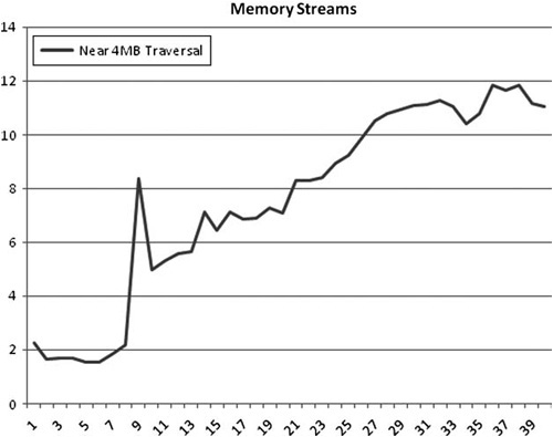
Figure 6.4. The number of arrays we are reading concurrently changes our performance. On this Intel Xeon, there is a significant penalty reading above eight streams. We traversed slightly less than 4MB, because parsing exactly 4MB causes a different cache penalty. The source for this chart is available in the perf Test Harness test “memory/stream/memorystream.”
So what is the conclusion? In the quad-core 3Ghz Intel Xeon used in the test, hardware pre-fetching will suffice when you have fewer than eight memory arrays streaming per processor. The more streams you use, after eight, the worse your performance will be. (Again, this number can and will differ from processor to processor, so you will want to do your own tests on your target hardware.)
An important side note: We chose arrays slightly smaller than 4MB for several reasons. One, it is slightly smaller than an OS memory page. This is important because many hardware pre-fetch implementations do not allow more than a single stream per page (Intel, 2008). Unfortunately, iterating at a stride of exactly 4K causes problems with the cache on our test systems. This issue is discussed more in the “Fix Critical Stride Issues” section of this chapter.
Layout of memory is crucial, and one way to maximize linear access through memory is to choose the appropriate data structure. There are two major possibilities for laying out memory.
Typically, we create array of structures (AOS). They take the following form:
struct aos
{
     float m_Float1;
     float m_Float2;
     float m_Float3;
     float m_Float4;
};

aos myArray[256];
AOS is used in a lot of scenarios. Most APIs organize their data this way. OpenGL is notable in supporting both AOS and SOA.
The other, somewhat less popular format, is a structure of arrays (SOA):
struct soa
{

     float m_Float1[256];
     float m_Float2[256];
     float m_Float3[256];
     float m_Float4[256];
};

soa myArray;
The difference is subtle. They both hold the same amount of data, and they are functionally equivalent. Why choose one structure over the other?
In Figure 6.5, you can see the effect of each structure in memory. Interleaved memory, like the AOS, would be appropriate if you were planning to iterate through every member and every iteration. But what if you were only going to iterate through one member at a time?
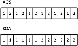
By using the array of structures and iterating through only one member, you are much closer to periodic access. If you use the structure of arrays and iterate through one member, your access pattern is more similar to linear than periodic.
Understanding the difference between AOS and SOA is helpful when writing multi-threaded code as well. We will discuss this in Chapter 13, “Concurrency.”
When using an AOS, you can still make some accommodations for better cache usage. When you strip mine, you split iteration of single members (periodic access) into cache-friendly chunks. This technique increases both temporal coherence and spatial locality.
Consider the following code:
for( int i=0;i<numStructs:i++ )
{
      m_Vertex[i].pos = processPos(&m_Vertex[i].pos);
}

for( int i=0;i<numStructs:i++ )
{
      m_Vertex[i].normal = processNormal(&m_Vertex[i].normal);
}
As the first loop iterates, the automatic hardware pre-fetch will fetch data in anticipation of its use; if the loop is large enough, later parts of the loop may evict values fetched earlier. If the evictions occur, the second loop will not benefit from the first loop’s use of the cache.
A solution is to perform both loops together using blocks of access and performing memory loads on both members. This is called strip mining.
for( int j=0;j<numStructs;j+=blocksize)
{
      for( int i=j;i< blocksize;i++ )
      {
            m_Vertex[i].pos = processPos(&m_Vertex[i].pos);
      }
      for( int i=j;i<blocksize;i++ )
      {
            m_Vertex[i].normal = processNormal(&m_Vertex[i].normal);
      }
}
Much better. Now the first loop is warming the cache for the second loop and an increase in overall performance occurs. The optimal block size can differ from processor to processor because cache size is not standard.
Allocate memory with the new operator, add a local function variable, add a static global variable; to an application developer it may all seem like homogenous memory, and in some ways that is true, but the low-level implementation details expose nuances that help you make decisions.
When you step into a function, instructions push the parameters onto the stack; any variable whose scope exists within the function will be placed on the stack as well. As you load, store, and calculate values within the function, they are likely to remain in the cache because the stack maintains proximity. When a function returns, you are simply moving down the stack.
The stack has the advantage of maintaining spatial locality and temporal coherence. It is always in use, so it tends to stay in cache. Data is grouped well, since all the data used by a function is adjacent.
Of course, stack space is finite. Especially when working with recursive code, minimizing stack usage is important because it will give you better performance.
Global memory is memory that is allocated as part of your program image. Static and global variables are stored here, the only difference being the scope. Global memory is not freed until your program closes, which is a great way to eliminate memory fragmentation—a common cause of cache misses due to a lack of locality.
Typically, the linker allocates global memory based on the order that the linker receives object files. Therefore, items that are frequently accessed together may benefit from being in the same linkage unit (i.e., same .cpp or .c file for C/C++ developers) in order to preserve locality. It can also be possible to specify explicitly where in the image globals are allocated. Check with your specific compiler to see how it handles global variables. Things like profile-guided optimization could affect variable order, too.
One important caveat about sharing global variables occurs when you are accessing variables with multiple threads. Variables that are co-located in memory may suffer performance due to a synchronizing performance problem called false sharing. For more on false sharing, see Chapter 13.
Memory created or freed dynamically uses the heap. For C++ developers, this typically involves a call to new or delete. C developers will be familiar with malloc and free. Heap memory is subject to fragmentation over time, based on the allocation pattern, although memory managers work hard to minimize this, which is in itself a possible source of performance loss.
Allocating and freeing memory has a high cost relative to heap or global memory. Memory managers can be very complex. Although the average case can be cheap, sometimes the memory manager will have to request memory from the operating system, reclaim memory from a free pool, or perform other bookkeeping optimizations. These can sometimes be quite costly.
However, when you need dynamic memory, that’s a cost you have to pay, but there are many tactics that can help reduce the costs of dynamic memory.
Your authors once sat in on a lecture given by a recent graduate where he discussed topics about the game industry that surprised him in his first days on the job.
On one of his first days writing code, he decided to dynamically allocate memory using the new operator. To his surprise, the keyword caused a compile error. Surprised by his results, he sheepishly asked his boss.
“How do I allocate dynamic memory?”
“You don’t,” replied his boss.
The company’s policy was to remove the new operator and only statically allocate. For devices with limited resources, this can be very effective. But it is quite limiting. Most modern games require dynamic memory management in order to move memory usage from system to system as gameplay changes.
Is there any performance difference between accessing statically allocated memory versus dynamically allocated memory?
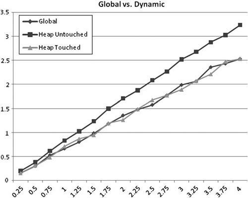
Figure 6.6 shows the differences between traversing static allocation and the three access patterns. Notice that dynamically and statically allocated memory achieve very similar performances. Heap Untouched includes data that is slower due to lazy allocation. To ensure that dynamic memory achieves the same performance as global, iterate through the array immediately after allocating the array.
Consider a particle system. The particles are modeled using many small structs in some sort of list structure. This data is traversed at least once a frame, maybe more if separate passes for position update and rendering happen.
In the case of a particle system, dynamically allocating particles from the heap can lead to several problems. First, since the structures are small, they may cause fragmentation. The second and much bigger problem is that since they are being allocated dynamically, they can lead to a random access pattern.
If you keep the structs in an array, so that they are always in linear order, you can gain two benefits. First, memory allocation activity is reduced. You always order the array so that “active” particles are at the front. When a particle is freed, you place it at the end of the array and swap the last “active” particle with the now-dead particle in the array. This divides the array into two regions—active particles up front and dead particles at the end.
When you allocate a new particle, you just “reactivate” the first dead particle. You only grow the array when adding more particles. For a continuous particle effect, like spray from a waterfall, this will result in the array growing and staying steady in size. No more allocations and linear access will lead to overall fast performance.
The array approach works less well when the working set varies wildly. For instance, an explosion effect might grow to a high number of particles and then ramp back down. The array approach can be wasteful because most of the time it will be allocating more memory or holding onto more memory than is needed. If you keep a lot of memory in systems that use this approach, you can end up wasting it.
Reduce, reuse, recycle! Pooling is designed to maximize efficiency when you are dealing with lots of similar objects. The idea is simple: Maintain a large pool of memory that holds many copies of the same thing. With our particle example, you would allocate, say, a thousand particles up front in a contiguous array. Instead of dynamically allocating particles, you get a free instance from the pool. When you are done with the particle, you return it to the pool.
This is helpful for several reasons. Since all particles are in the same area of memory, the working set will tend to be more coherent (although rarely fully linear). Memory fragmentation will not occur, because the particles aren’t being allocated in the same memory space as objects of other sizes.
Most significantly, pooling can be very helpful when the allocation costs are high. Particles are usually lightweight; however, you may find that other items are more complex. If setup costs are high, then pooling objects and not fully destructing them between uses can save a lot of time.
POS—plain old structures—are structures with no constructor or destructor.
Suppose that you allocate an array of a million points to store mesh data in. The point class has a constructor, which sets its position to some safe value, like (0,0,0). You immediately overwrite these values with data from a file.
The performance problem here is that when the array is allocated, the constructor will be called on each instance. So before you can load data from the file, you have to wait for a million points to get values set on them so they can be immediately overwritten with real data.
If you can avoid these destructor/constructor calls, you can save a lot of time.
Carefully defining the scope in which memory is needed can lead to opportunities for optimization. Many times, code needs to allocate temporary storage. The lifespan of the storage may be just for the duration of a function call or a single frame of rendering.
Often, this temporary data is simple data that does not need to be destructed. For instance, points or primitive types, or pointers that only point to other data in the temporary pool, are all things that can be torn down without destructors being called.
Many games implement pools for the lifetime of the current level. Everything related to the level is allocated from this pool, and when the level needs to be unloaded, the pool is simply discarded, all at once.
Another useful trick is a frame allocator, so named because it gives out memory that is only valid for a single frame (or less). This is a stack from which memory can be allocated on demand. At the start of a function, the position in the stack is noted. Code is executed, and memory is allocated from the frame allocator contiguously. Before the function returns, the stack pointer is reset to where it was at the beginning of the function. At the end of each frame, the stack position is reset to zero.
The allocator is nice because it gives very fast allocations and even faster deallocation. It can be compatible with types that have constructors, but destructors won’t be run.
Alignment can be an issue with this (and other) custom allocation schemes. For more information on memory alignment see Chapter 4’s discussion on “Alignment and Fetching.”
The best way to understand memory performance is to do some simple experiments. The next several sections will do just that.
Pointer aliasing occurs when two pointers reference the same address. This is a perfectly acceptable practice, but if the compiler can’t rule out the possibility for two pointers to “alias” to the same location, it has to be conservative with its optimizations, typically reloading data from memory more than is needed.
The following test uses two pointer references to the same address.
void func( int a[], int *p )
{

      for( int i=0; i<ARRAY_SIZE; i++ )
      {

            a[i] = *p + 5;
      }
}
If the compiler can’t rule out aliasing, then it has to implement this function by loading *p from memory every time through the loop.
If aliasing is not a risk, then the loop can be optimized. In fact, Visual Studio 2008 implements it with a rep stos instruction, the same as a memset call.
When tested on our standard machine, the unaliased version of the function was roughly 30% faster than the aliased version.
How does the compiler determine when it has to worry about aliasing? Ultimately, it can only make a best guess, and it has to guess conservatively to ensure that the program will work. Some compilers provide keywords for indicating assumptions about aliasing, either that two pointers are not aliased or that they are. For instance, in GCC, you can use _restrict_ to indicate this, while Visual Studio uses _restrict.
If you aren’t sure, check the assembly. It will be obvious if the compiler is being careful about aliasing because there will be a lot of extra load and store operations.
Your compiler by default will align structures to their natural alignment by padding with extra bytes. A structure’s natural alignment is the alignment of the largest member. For the following structure, which has a double, the natural alignment is eight bytes, which is the size of an IEEE double-precision float.
struct eightByteAligned
{
     float m_Float;
     double m_Double;
};
Members within a struct are also aligned to their natural alignments. For instance, in eightByteAligned, m_Float will be aligned to an eight-byte boundary because it is at the start of eightByteAligned. There will be four bytes of padding and then m_Double. As a result, eightByteAligned will be 16 bytes long despite only containing 12 bytes of data. Figure 6.7 illustrates some different layout possibilities.
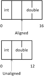
Figure 6.7. Example of possible alignment of a float and double with four bytes’ padding (top) and without padding (bottom). Your compiler may have its own approach to this situation.
You can use various compiler options to change alignment and packing rules. Sometimes, you may want to pack a structure for minimum space usage, while at other times for best alignment.
Unfortunately, the compiler has less control over alignment at runtime. For example:
//function prototype
char* getData();
int* array = (int*)getData();
If the function getData() returns a char array, it will be one-byte aligned (meaning any address), therefore, the array has a one–in-four chance that it will be four-byte aligned. If the char happens to be on a four-byte multiple, all is well. Figure 6.8 demonstrates the performance difference this can cause.
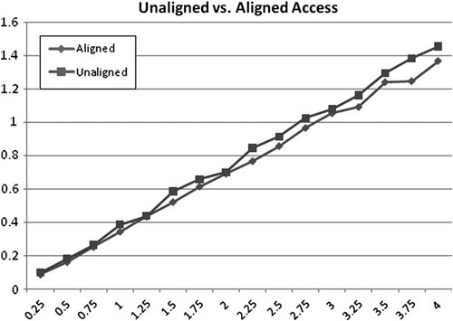
Figure 6.8. Performing addition on 4MB of integer operations shows a slight performance difference between aligned and one-byte offset unaligned data.
If it is not, then depending on platform, OS, and compiler, there will either be a loss in performance or an error. If you have to cast data a certain way for things to work, that’s fine, but be aware that it’s not optimal.
Most CPU caches are set-associative. (A set-associative cache can choose to map a given address to one of N locations.) A set-associative array can have problems when accessing data at certain strides. Similar to how some engine speeds can cause parts of your car to vibrate, these critical strides impact performance by causing the cache to act against itself.
The worst-case critical stride is equal to (number of sets) × (size of cache line).
Consider an Intel Core 2 Duo with an L2 cache size of 2MB. The Core 2 Duo uses cache lines of 64 bytes and is eight-way set-associative.
Therefore, we have 2,048KB/64 bytes = 32,768 cache lines of L2 cache.
These 32,768 lines are organized into eight ways, which gives us 32,768 lines/8 ways = 4,096 total sets.
If you were to have a large array of data, and iterate over 64-byte items at a stride of sets × cache line size = 4,096 × 64 bytes = 262,144 bytes, you would only be using eight L2 cache lines for your traversal. Instead of being able to access 2MB of data before blowing the cache and having to fetch from main memory, you would only be able to access 8 × 64 = 512 bytes!
Now, a 262KB stride is a pretty specific scenario, but critical strides can affect you in more pedestrian situations as well.
Consider a one-channel texture that is 4096px on a side with 1 byte-per-channel. In other words, pixels equal bytes. If you were to traverse the first column of this texture, you would load a byte every 4,096 bytes. The first byte of each column won’t share the same set, but the first pixel of every 64th row will.
To see this more clearly, consider the math involved in deriving a set from an address.
For simplicity’s sake, let’s assume our texture begins at address 0 × 0000. Since addresses are typically represented in hex, we will do the same. Remember 64 bytes in decimal is 0 × 40 in hex and the number of sets for this example 4,096 in decimal is 0 × 1000.
To derive the set, use the following formula:
set number = (address / line size) % numsets
For address zero, it is obviously set zero, but let’s try a more challenging address. Consider the address 0 × 40000.
0 × 40000/0 × 40 % 0 × 1000 = 0 × 0
Where does the critical stride come in? The address 0 × 40000 is the first pixel of the 64th row of the texture, and shares the same set as address zero. This is an example of critical stride. By fetching the first text in row 0 and then the first texel in row 64, you have used two out the eight ways for set zero. If you were to continue with this stride, addressing 0 × 80000, 0 × 120000, and so on, you would quickly use all eight sets. On the ninth iteration with that stride, a cache line eviction must occur.
Because of how the cache is implemented, this is the worst case. Instead of having 2MB of cache available, you’re down to 512 bytes. This leaves pre-fetching with very little room to compensate for slow memory. Similar issues occur with other large power-of-two strides, such as 512, 1,024, and 2,048. Figure 6.9 shows the performance of critical stride scenarios.
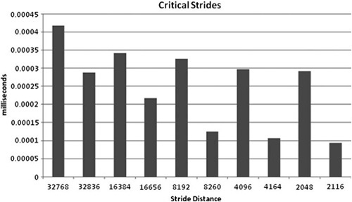
Figure 6.9. Average load time equals total time/number of loads. The source code for this test is available in the Performance Test Harness: “memory/criticalStride.” These values will vary significantly, depending on the amount of data traversed and the architecture of your cache.
The best solution for this kind of problem is to pad your data to avoid larger power of two strides. If you know you are only reading memory once, as occurs when streaming music, you can use advanced SSE instructions.
Doing one thing at a time faster is good. Doing four (or more) things at the same time is even better. For game developers, that is the basis behind using 128-bit SSE instructions. SSE instructions are an example of SIMD, or Single Instruction Multiple Data, operations. By using SSE instructions, you have access to special hardware that can perform operations in parallel.
Beyond Math with SSE
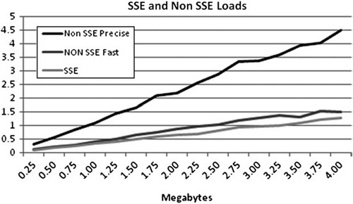
Typically, we think of SSE instructions as ways to increase math performance, but can SSE instructions offer a boost to memory fetching as well? It’s difficult to tell by looking at the following chart in Figure 6.10. Without examining the trade-off of performance vs. accuracy, there is no way to compare apples to apples.
You can also use SSE instructions to provide software pre-fetching. By using software pre-fetching, developers can hint to the memory system in advance of the actual access. Pre-fetching preloads one cache line at a time. When using software pre-fetch calls, developers should, when possible, utilize many loads per software pre-fetch since cache line pre-fetch is not a computationally free instruction.
One way to implement SSE instructions is to use intrinsics, which compile to specific assembly instructions. The intrinsic call_mm_prefetch( char *p, int i ) provides four different types of pre-fetch enumerations:
_MM_HINT_T0: Pre-fetch data into all cache levels_MM_HINT_T1: Pre-fetch data into level 2 cache, but not level 1_MM_HINT_T2: Pre-fetch data into level 3 cache, but not level 1 or 2_MM_HINT_NTA: Nontemporal access, loads directly to level 1 cache bypassing other caches
At the very least, we can suggest that use of software pre-fetch requires special care and testing across many processors to ensure reliable performance increases across all processor versions. A simple alternative to using software pre-fetching is to use an access pattern such as linear access forward or backward to ensure best-case use of automatic hardware pre-fetch.
For more information on computing with SSE, see Chapter 8, “From CPU to GPU.”
Accessing memory on a device across the bus from the CPU is problematic. Even if the device’s bandwidth is adequate, the bus is even slower to serve requests than main memory. If you are, for instance, updating a vertex buffer in GPU memory, reading data back can introduce significant delays because of the extra roundtrips over the bus.
For this reason, write-combining is implemented. Busses are most efficient when large, contiguous chunks of memory are written; small writes, or interspersed reads and writes, can be much slower. To keep writes big and fast, write-combining buffers are provided in the CPU. If data is written contiguously, then it is cached in the buffer until it can get sent all at once.
A practical example is shown here. Consider the following 32-byte vertex:
struct Vert
{

     float m_Pos[3];
     float m_Normal[3];
     float m_TUTV[2];
};
If you were to update this vertex, if it were a point sprite in a dynamic vertex buffer, would the following code seem appropriate?
for( int i=0;i<numVerts;i++ )
{

      vertArray[i]. Pos [0] = newValueX;
      vertArray[i]. Pos [1] = newValueY;
      vertArray[i]. Pos [2] = newValueZ;
      vertArray[i].m_Norm[0] = vertArray[i].m_Norm[0];
      vertArray[i].m_Norm[1] = vertArray[i].m_Norm[1];
      vertArray[i].m_Norm[2] = vertArray[i].m_Norm[2];
      vertArray[i].m_TUTV[0] = vertArray[i].m_TUTV[0];
      vertArray[i].m_TUTV[1] = vertArray[i].m_TUTV[1];
}
Write-combined memory is uncacheable, and doesn’t travel through your memory system the way you may be accustomed to. Reads are done from system memory into the L1 cache. Writes are also handled differently. Instead of writing directly back across the bus, they are put into the write-combining buffers.
In the P4 processor, for example, you have six write-combined buffers that are each 64 bytes and act similarly to a cache line. When you update only the position, you are causing partial updates to each write-combined buffer. For example:
       vertArray[0].m_Pos[0]=1;
       vertArray[0].m_Pos[1]=2;
       vertArray[0].m_Pos[0]=3;
       vertArray[1].m_Pos[0]=4;
       vertArray[2].m_Pos[1]=5;
       vertArray[3].m_Pos[2]=6;
This would produce the following write-combined buffer (unwritten addresses are represented by dashes), as shown in Figure 6.11.
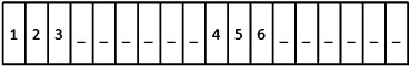
Figure 6.11. Updating only the changed values in 64 bytes of memory that map to one write-combined buffer.
If you were to touch every address, including those whose value you don’t update, it would produce a different write-combined buffer and would look like the following example shown in Figure 6.12.
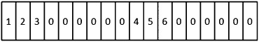
Figure 6.12. Updating and touching changed and unchanged values in 64 bytes of memory that map to one write-combined buffer.
Note that this implementation updates every address.
Now here is where the performance difference occurs. As stated earlier, we have six write-combined buffers in the P4. As we write back values, they are first written to a write-combined buffer. When all of the buffers have been exhausted, a previously used buffer must be evicted.
The rules of eviction are as follows: If you update the entire buffer, a 64-byte burst copies the data across the front-side bus. If the buffer is not completely modified, then the eviction occurs using 8-byte increments.
To recap, from the perspective of writing to nonlocal video memory, it is faster to update all values of the write-combined buffers than it is to partially update the write-combined buffer.
Most applications don’t spend a lot of code writing to the GPU. Usually, there are just a few key routines that deal with it. However, if written poorly, those routines can become a major bottleneck. Getting them right is important.
You can also make the GPU update itself, using geometry shaders or render-to-vertex-buffer operations.
Finally, some motherboards or hardware configurations result in write-combining being disabled. If you are doing a lot of profiling, you should make sure it’s enabled before optimizing to take advantage of it.
Memory access patterns are a huge part of application performance. While learning all the tricks can take a long time, the basics aren’t too complicated. Be sure to keep the following elements in mind:
Measure, measure, measure. The figures in this chapter will differ from processor to processor.
You will never eliminate all cache misses. But you can reduce them.
Memory system specifics vary from processor to processor. Make sure to measure performance on the hardware your users will be using.
Do what you can to both conserve memory and access it linearly. Linear access of contiguous, efficiently packed memory is the fastest option.
Remember, at some point you will reach a physical limitation that will be hard to overcome. Even cached memory takes time to read.
When this happens, don’t forget that the fastest memory is the memory you don’t touch—look for an algorithmic-level optimization that is cache friendly and reduces memory access. If your working set is small enough, you won’t need any of the techniques we’ve discussed in this chapter.