What is your favorite optimizing compiler? Have you even heard of an optimizing compiler? Back in the day, you would have had a compiler, and then, if you so desired you might have bought a better compiler that would perform optimizations. Now, it’s likely that the compiler you own does plenty of optimizations—even free compilers do. Today’s compilers perform very robust optimizations, such as link-time optimizations that optimize between object files.

If you want to start an argument, you could discuss either politics in a D.C. bar or micro-optimizations in a blog. As you will recall from Chapter 1, micro-optimizations are detail-oriented, line-by-line performance work. Hand-writing assembly, tweaking the order of specific operations, and the like all fall under this umbrella.

A program in a high-level language like C++ has many layers of abstraction above actual hardware operations, which is great since coding at the hardware level is hugely inefficient. The compiler converts C++ code into machine code that the processor converts into micro-code at runtime. Because of this, the net effects of changes on an individual line of code are difficult to predict without also knowing the exact compiler version, settings, and processor used to run the program.

Let’s use the perf Test Harness test “compute/loopunrolling/unrolledEF” and vary the compiler settings on our copy of Visual Studio (any version from 6 on) to illustrate how the compiler’s assembly can vary. Using the fast floating-point model (/fp:fast) yields significantly different assembly than if we used the precise floating-point model (/pf:precise).

The x86 architecture can do floating-point math in 32-, 64-, and 80-bit mode, and setting the compiler’s floating-point model controls both how the internal CPU precision is set, as well as whether or not extra instructions are added to perform explicit rounding or error checking. Compare the assembly listings in Listing 7.1.

// fp:precise
fld   dword ptr [eax-4]
add   eax,10h
sub   ecx,1
fadd  dword ptr [esp+8]
fstp  dword ptr [esp+8]
fld   dword ptr [esp+4]
fadd  dword ptr [eax-10h]
fstp  dword ptr [esp+4]
fld   dword ptr [eax-0Ch]
fadd  dword ptr [esp+0Ch]
fstp  dword ptr [esp+0Ch]
fld   dword ptr [eax-8]
fadd  dword ptr [esp+10h]
fstp  dword ptr [esp+10h]

// fp:fast
fld    dword ptr [eax-4]
add    eax,10h
sub    ecx,1
faddp  st(3),st
fld    dword ptr [eax-10h]
faddp  st(2),st
fadd   dword ptr [eax-0Ch]
fld    dword ptr [eax-8]
faddp  st(4),st
fstp  dword ptr [esp+10h]

As you can see, the floating-point model has a big impact on how much work gets done and in what way—in precise mode, our snippet has eight stores/loads. Fast mode does half as many. Not bad for changing a flag.

The code in the performance test “compute/fp_model” generates the previous assembly. Running the test in precise and fast mode shows that the flag can make a significant difference. On a test machine, the precise mode was 3.17 times slower than fast mode.

This example provides you with a simple example to understand how a micro-optimization may yield performance gains. More examples of micro-optimizations, and specifically floating-point optimizations, can be found throughout this entire chapter.

When you find that your application is CPU bound, the next step is to determine whether you are compute or memory bound. You will want to use a profiler that can read the CPU counters to do this; see Chapter 4 for an overview of tools. Chapter 6’s “Detecting Memory Problems” section discusses how you can distinguish between memory and compute bound applications.

Basically, if your application is CPU bound and not bound by memory or instruction fetching, it is bound by computation. You can confirm this by looking at the code identified as a hotspot. If it is doing a lot of arithmetic operations, not loads or stores, you are probably looking at a computational bottleneck. If the number of cache misses for the suspicious code is low, that’s another supporting condition.

Optimization has been described as the art of trading time against space in the search for speed. Lookup tables (and related techniques) are the most direct instance of this trade. They trade memory for performance by storing the results of calculations in memory and doing a lookup in the table instead of performing the calculation.

The classic lookup table example is speeding up sin/cos. Many older games didn’t require high accuracy in their trigonometric equations, so they would approximate sin/cos in, say, 1,024 steps by having an array 1,024 entries long containing precalculated values. Then when they needed to calculate sin/cos, they would simply look up in the table, saving a lot of computation.

Unfortunately, the gap between memory fetch performance and calculation has only grown. As a result, lookup tables are less often the obvious choice for performance.

If the penalty of cache misses exceeds the performance gain from skipping the calculations, then the lookup table is useless. Fetching calculations from a large table may evict other values, resulting in compulsorily cache misses for upcoming instructions. It’s likely that the use of a lookup table will result in a random memory traversal pattern, which we learned in Chapter 6 is a bad case for automatic hardware pre-fetching and is likely to cause frequent cache misses.

The best case for lookup tables is when they are small enough to stay cache resident, and then they can save you a large amount of computation. Use a lookup table when the table is small, when access to the returned calculations maintains spatial locality, or when the amount of calculation saved is worth the price of cache misses. In other words, you should test your lookup table’s performance compared to simply calculating the values you need. Make sure to take into account varying cache sizes of different hardware targets.

An alternative to lookup tables is memoization. Memoization is a specialized form of caching that stores the results of computations for reuse. In both approaches, you end up with a table storing results you can quickly look up, but memoization generates that table dynamically.

The basic idea behind memoization is that when you complete a calculation, you make a “memo” to yourself noting the inputs and outputs of the calculation. For instance, suppose that you wanted to calculate the Fibbonaci sequence. Each successive number in the Fibbonaci sequence is made up of the sum of the previous two numbers. Or more mathematically:

     F(0) = 0
     F(1) = 1
     F(n) = F(n-1) + F(n-2)

Suppose that you implemented this by using a simple recursive function that computes the Nth value.

int fibonacci(int n)
{
     if(n==0) return 0;
     if(n==1) return 1;
     return fib(n-1) fib(n-2);
}

This will give you the correct results, but very slowly since there are many function calls and redundancy. You can speed things up quite a bit by using memoization.

map<int, int> fibonacciMemos();

int initialize()
{
     fibonacciMemos[0] = 0;
     fibonacciMemos [1] = 1;
}

int fibonacci(int n)
{
      // Check for a memo about this number.
      map<int,int>::iterator i = fibonacciMemos.find(n);
      if(i == fibonacciMemos.end())
      {
         // Calculate the fibonacci number as we would normally.
         int result = fib(n-1) + fib(n-2);
         // Store the result for future use.
         fibonacciMemos[n] = result;
         // And return.
         return result;
      }
      // Look it up and return.
      return fibonacciMemos[n];
}

The performance gains you see are dependent on the time it takes for the memory reads vs. the time involved in the calculation. If the memory lookup you create (the map in the above example) is hardware cache friendly, the savings will almost always validate the effort of implementation. For an example of an ideal memory lookup for memorization, refer to the perf-TestHarness test “compute/fibonacci.” The memoization example in this case is ideal, and the performance increase is in the hundreds of percents. Your mileage on other memoization opportunities may vary depending on the cache friendliness of your requests.

A common extension to this technique is to cap the memo storage space, making it a cache. For instance, perhaps only the most recently accessed 1,024 memos will be kept. This is useful for more complex calculations that can give larger results. You will want to profile carefully to make sure that you are striking the right balance of cache vs. calculation.

Another useful technique is to make memoization work with larger or more numerous input parameters. A key gating factor on the performance of memoization is the cost of looking up the right answer. If you have a hundred string parameters, it might become very costly to do this. There are many solutions, but the most common ones are either nested hash tables or combining the multiple input parameters into a single key that supports quick comparisons. Make sure that you handle collisions correctly in the latter case.

A practical example of memoization is the post-TnL cache on the GPU, which we’ll discuss in Chapter 9, “The GPU.” This cache significantly reduces the number of times the vertex shader must be run.

The goals of abstraction and performance often conflict. An abstracted codebase will have lots of little functions and classes, which can make it easier to extend and maintain, but it will cost in performance because of the overhead of making lots of little function calls. Removing a little abstraction in a compute bound routine can pay big dividends.

Function inlining occurs when the compiler (or developer) takes the body of a function and replaces calls to that function with direct execution of the body code. For example:

int cube(int i){return i*i*i;}
int main(int argc, char* argv[])
{
    for(int i=0; i<100; i++)
       printf("%d
", cube(i));
}

Could be rewritten as:

int main(int argc, char* argv[])

{
    for(int i=0; i<100; i++)
        printf("%d
", i*i*i);
}

This is beneficial since calling a function has overhead. It depends on your calling convention, but function calls commonly include the following steps:

With function inlining, these steps are eliminated or reduced, and the CPU can spend its time doing productive work rather than doing bookkeeping. In addition, inlining can offer more opportunities for the compiler to optimize code, since it can mix the inlined code with the surrounding function’s code for better performance.

Sounds good, but similar to other optimizations, there are some catches. First, bear in mind that function inlining is another space vs. time trade-off. Instead of having a single block of machine code for that function that everything jumps to, you are essentially replacing the few bytes it takes to call that function at each call site with the actual machine code implementation of the function. This increases executable size, which isn’t necessarily bad by itself (people have lots of RAM and disk space), but carries another, more subtle problem.

Inlining increases the working set of instructions, which means that there is effectively less room in the instruction cache, because it has to store duplicates of the same code.

Of course, inlining by hand is a huge maintenance nightmare. It makes a lot more sense to let the compiler do it, which it will generally do on its own when it feels inlining makes sense. You can also hint that you’d like a method or function to be inlined by using the inline keyword.

How compilers handle inlining differs, so let’s use the Visual Studio 2008 compiler documentation to explore how Microsoft’s compiler interprets the standard.

There are two major decisions a compiler must make before inlining a function. First, it performs a cost/benefit analysis. Among other things, this is based on the size of the function to be inlined. The best candidates for inlining are functions that are small, fast, and called frequently from only a few call sites. If the compiler believes this code would be faster left as a function call, then inlining does not occur.

There are also some situations where inlining isn’t readily possible. For instance, if a virtual function is called in a situation where the specific type cannot be inferred, then the function cannot be inlined (since the specific implementation will only be known at runtime). Function pointers also invalidate inlining attempts for a similar reason.

Recursion is incompatible with inlining, since the compiler would have to either solve the halting problem or produce a binary of infinite size. (Turing introduced the halting problem, but Stroustroup noted that inlining recursive code requires that the compiler solve it.) There’s typically a small laundry list of cases for every compiler where inlining is not possible. Check the compiler docs for details.

If all these conditions are met, the function will be inlined.

You can use the __forceinline keyword to disable the cost/benefit analysis and force a function or method to be inlined whenever possible, subject to the restrictions mentioned previously. This compiler heuristic is pretty good, so unless you have strong performance numbers to back it up, don’t go sprinkling __forceinline around your codebase, because it’s liable to hurt more than it helps.

In general, the guideline with inlining is to let the compiler deal with it unless you can find evidence that you need to step in.

#define cube(x) (x)*(x)*(x)

inline int cubei(int i){return i*i*i;}

int main(int argc, char* argv[])
{
     int i=0,j=0;
     int k = cube(++i);
     int l = cubei(++j);
     return 0;
}

Out-of-order execution allows you to have multiple instructions in flight at the same time. Parallel execution can give major performance wins. However, it does complicate something, namely branching.

Branches come in two varieties: conditional and unconditional. Unconditional branches are easy to handle; they always jump to the same instruction, no matter what. As a result, they don’t affect out-of-order execution.

Conditional branches, however, pose a problem. The branch can’t be taken until any instructions that affect the decision are finished executing. This introduces “bubbles,” periods of halted execution, in the execution pipeline. Instruction reordering can help to avoid bubbles, but it’s still a problem.

To get around this, most CPUs predict which way the branch will go, and start speculatively executing based on the prediction. Some branches will be hard to guess, but a lot of them look like this:

for(int i=0; i<100; i++)
    doWork();

In 99 out of 100 times, the branch in this loop is going to repeat. A lot of the time, branches will always go the same way. If the CPU only guessed that the branch would go back for another loop, it would be right 99% of the time—not bad for a simple strategy!

If the CPU mis-predicts a branch, it just discards whatever work it guessed wrong and carries on. This wastes a little bit of work, but not much, because a branch prediction miss is roughly equivalent to the depth of the CPU pipeline (Intel Software Optimization Guide). A successful branch prediction is free, like on the P4, or very low, like predicted, taken branches on the Pentium M.

The processor’s ability to predict a branch is dependent on the branch prediction algorithm the processor uses and the predictability of the branch. Generally, the less random a condition is, the less likely the processor will miss a branch. Some processors can support periodic patterns for branch prediction, while others will not. A condition that is 50% randomly true or false is completely unpredictable and likely to cause the most branch prediction misses. Branch prediction often uses a branch target buffer to store historical data on which way branches have gone. This can give a major accuracy improvement for predictions.

After you’ve identified a hot spot that is bottlenecked by branch mis-predictions, there are several techniques you can use to help reduce misses. The cost of a single cache miss is many times greater than a branch mis-prediction, so make sure that you have correctly identified your bottleneck.

What can you do to help reduce prediction misses? The following sections discuss this issue.

if( condition[j]>50 )
      sum+=1;
else
      sum+=2;

myArray[i]=rand()%100;

myArray[i]=rand()%10;

if(a) z = c; else z=d;

z = a*c + (1-a)*d;

Back before compilers would unroll a loop for you, programmers noticed that unrolling a loop achieved better performance than leaving it rolled. Let’s start by explaining what loop unrolling is via a simple example:

int sum = 0;

for( int i=0;i<16;i++ )
{
      sum +=intArray[i];
}

This loop will execute 16 times. That means that you will have 16 addition assignments and 16 iterator updates. You will also execute 16 conditional statements. For every iteration of the loop, you must perform a conditional branch and an increment.

Unrolling this loop might look like this:

int sum=0;

for( int i=0;i<16;i+=4 )
{
      sum+=myArray[i];
      sum+=myArray[i+1];
      sum+=myArray[i+2];
      sum+=myArray[i+3];
}

This version appears to dedicate more cycles to work (addition) and less to the overhead of updating the loop. The key word here is “appears.” The compiler does some interesting things behind the scenes.

Your compiler is looking for opportunities to enhance performance, and when it finds those opportunities, it rewrites the code behind the scenes to make it faster and better suited to the CPU. These two snippets of code generate the same assembly in Visual Studio 2008 (although different settings may generate different code). Their performance is identical (see Listing 7.2).

//unrolled Loop
mov  esi,dword ptr [eax-8]
add  esi,dword ptr [eax-4]
add  eax,10h
add  esi,dword ptr [eax-0Ch]
add  esi,dword ptr [eax-10h]
add  edx,esi
sub  ecx,1
jne  unrolledLoopPerfTest::test+14h (419EF4h)

//Rolled Loop
mov  esi,dword ptr [eax-8]
add  esi,dword ptr [eax-4]
add  eax,10h
add  esi,dword ptr [eax-0Ch]
add  esi,dword ptr [eax-10h]
add  edx,esi
sub  ecx,1
jne  rolledLoopPerfTest::test+14h (419EB4h)

Intel’s “The Software Optimization Cookbook”^[1] suggests the following optimization to the unrolled loop. It reduces data dependencies, which allows for more instruction level parallelism.

int sum=0,sum1=0,sum2=0,sum3=0;

for( int i=0;i<16;i+=4 )
{
      sum+=myArray[i];
      sum1+=myArray[i+1];
      sum2+=myArray[i+2];
      sum3+=myArray[i+3];
}

sum =sum+sum1+sum2+sum3;

As you can see, the code is effectively doing four sums in parallel and then combining the results. If you check out Chapter 13, “Concurrency,” you will see how this approach leads naturally into true thread-level parallelism. It also leads to another valuable idea, that of SIMD instructions, such as SSE. It should be obvious how a single instruction that does four adds in parallel could be used to rewrite this loop.

One important wrinkle is dealing with leading and trailing data. This example is working with a fixed number of values. But what if it had a variable number of values to add? You could do any multiple of four with the previous loop, but you’d have to do something special to mop up the last 0-3 values:

int sum=0,sum1=0,sum2=0,sum3=0;

// Mask off the last 2 bits so we only consider

// multiples of four.
const int roundedCount = myArrayCount & (~0x3);
for( int i=0;i<roundedCount;i+=4 )
{
      sum+=myArray[i];
      sum1+=myArray[i+1];
      sum2+=myArray[i+2];
      sum3+=myArray[i+3];
}

sum =sum+sum1+sum2+sum3;

// Finish up the remaining values.
for(;i<myArrayCount;i++)
     sum += myArray[i];

For the trailing cleanup code, there are plenty of options to keep your speed up. For instance, you could use a switch statement and have cases for zero, one, two, and three remaining values. As long as you have plenty of values in myArray, the speed of the cleanup values won’t be a bottleneck.

But what if you’re using SSE and all the values have to be aligned? If you accept arbitrary arrays, there’s no guarantee that they will be aligned for SIMD. (You can usually assume that the floats will be at their natural alignment, meaning that if there are seven or more, there will be at least one SIMD-able block.) The solution is to have leading and trailing cleanup blocks that deal with the unaligned segments, leaving a big juicy chunk of aligned data for SIMD to churn through.

int sum=0,sum1=0,sum2=0,sum3=0;

// Deal with leading unaligned data.
int i=0;
while(i<myArrayCount)
{
     // Check to see if we can move to the aligned loop.
     if(isAligned(myArray+i))
     break;
     sum += myArray[i++];
}

// Fast, aligned-only loop.
for( int i=0;i<myArrayCount&~0x3;i+=4)
      AddSSE(myArray+i, counters);

// Finish up the remaining values.
for(;i<myArrayCount;i++)
     sum += myArray[i];

In Figure 7.1, you can see how good the compiler is at optimizing simple loops. The light columns are times for versions compiled without compiler settings turned on, and the dark columns are times for versions with compiler optimization turned on. As you can see, there is a marked improvement in unrolled enhanced floating-point performance and all integer implementations.

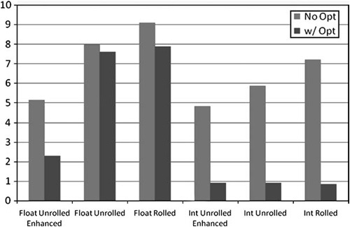
Figure 7.1. The differences between the different loop configurations are more apparent when optimizations are turned off. When turned on, implementations differ slightly on integers, but show a marked improvement on floating-point implementations. In other words, the compiler is able to analyze and optimize many of the loops to the same high level of performance despite the varying code. Time is in milliseconds.

Floating-point math has been a longstanding hot topic for game developers. At first, having it at all was out of the question. At best, you could do a few thousand integer operations per frame. As time went on, hardware-supported floating point became available, but it was still slow. Eventually, it became possible to do a lot floating-point operations (FLOPs) if you were careful to treat your compiler and hardware just so.

Nowadays, you don’t have to be quite as careful, but there are still some pitfalls. We’re going to go into them both as a practical matter and as an opportunity to show how compiler flags can affect runtime performance and behavior. Even if floats aren’t a problem for you, you’re sure to run into some compiler behavior down the line that is similar.

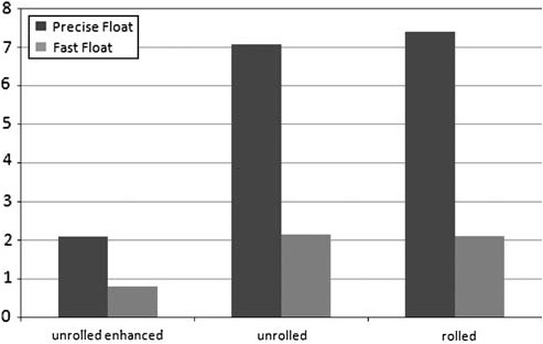
The compiler in Visual Studio 2005 and 2008 includes the ability to reduce the precision of floating-point operations for faster performance by setting the compiler option /fp:fast. (Note, you can also do this in the Code Generation page of the compiler settings.) Figure 7.2 shows the performance difference between these flags. The documentation for this capability explicitly points to video games as a good example where precision may not be the ultimate goal.

Figure 7.2. Floating-point model fast shows a significant performance increase over floating-point model precise for the loop unrolling floating-point tests.

When describing a CPU instruction’s performance, the two main characteristics are latency and throughput. Latency is the number of clock ticks a given instruction takes. For example, the latency of a floating-point multiply on the Pentium M is 5 clock ticks. Divide on the Pentium M is 18.^[2]

Throughput is always less than or equal to latency. For example, floating-point multiply throughput of the Pentium M is 2, which means that after 2 clock ticks, the execution unit can begin doing the next multiply. Divide’s throughput matches its latency at 18; therefore divide must finish completely before beginning the next. However, if you’re considering breaking out the instruction latency tables and optimizing your instruction order, think again. In most cases, the compiler will know more about the CPU than you do, and it will be able to automatically order the instructions as well or better than you can. Unless you are late in development and looking at a specific bottlenecked routine, it is probably not the right time to spend a ton of time optimizing for slow instructions. In fact, even if you insert inline assembly, the compiler will still often reorder it for better performance.

Make sure that you’ve checked the following things before jumping into assembly reordering:

With that out of the way, here are several techniques that can come into play when you start running up against slow floating-point performance.

if( distanceSquared > lodDistance*lodDistance)

int temp = *(int*)&floatVal;
temp -= FLOATING_POINT_ONE_POINT_ZERO;
temp >>= 1;
temp += FLOATING_POINT_ONE_POINT_ZERO;
return *(float*)&floatVal;

float InvSqrt (float x){
   float xhalf = 0.5f*x;
   int i = *(int*)&x;
   i = 0x5f3759df - (i>>1);
   x = *(float*)&i;
   x = x*(1.5f - xhalf*x*x);
   return x;
}

int rounded = (inNumber/4)*4;

int rounded = inNumber & ~3;

int divided = inNumber * 4;

int divided = inNumber << 2;

int divided = inNumber * variable;

X^=Y; Y^=X; X^=Y;

isFlagSet = someInt & MY_FLAG;

// Enums are a good place to store flags.
#define BIT(x) (1<<x)
enum
{
     FlagO = BIT(0),
     Flag1 = BIT(1),
     Flag2 = BIT(2),
     Flag3 = BIT(3),
}

// Example of setting and reading flags.
unsigned char flags = Flag1 | Flag3;
if(flags & Flag2) doSomething();

// We can clear a flag with by bitwise and-ing with the inverse of that flag.
flags &= ~Flag2;

// We can set a flag by bitwise or-ing it in.
flags |= Flag3;

// You can also clear/set/test multiple flags at a time:
flags |= Flag1 | Flag2;
flags &=~(Flag2 | Flag3);
if(flags & (Flag1|Flag2)) ifFlag1OrFlag2WereSet();
if(flags & (Flag1|Flag2) == (Flag1|Flag2)) ifFlag1AndFlag2WereSet();
if(flags & ~Flag3) ifAnyOtherThanFlag3WereSet();
if(flags & (Flag1|Flag2) == Flag1) ifFlag1IsSetAndFlag2IsNot();
if(flags == Flag1|Flag3) ifOnlyFlag1AndFlag3AreSet();
if(flags != Flag2) ifAnyConfigurationExceptOnlyFlag2IsSet();

// Some more advanced tricks:
if(~(flagA ^flagB) == (Flag1|Flag2)) ifFlag1And2AreDifferent();
if(flagA | flagB == (Flag2|Flag3)) ifBetweenAAndBFlag2And3AreSet();

X & 255; //is the same as X%256

X%Y = X&(Y-1) iff Y is a power of 2.

(X & 1) == 0; //is the same as X%2==0

(X ^(X >> 31)) - (X >> 31);

X ^Y>=0

unsigned int v; // compute the next highest power of 2 of 32-bit v
v-- ;
v |= v >> 1;
v |= v >> 2;
v |= v >> 4;
v |= v >> 8;
v |= v >> 16;
v++;

return v;

const float v; // find int(log2(v)), where v > 0.0 &&
            // finite(v) && isnormal(v)
int c;      // 32-bit int c gets the result;
c = *(const int *) &v;
c = (c >> 23) - 127;

return c;

Datatype Conversions

Processors natively support several different data types (signed/unsigned integers of various widths, half/single/double floats, SIMD formats, flags, etc). Because of this, data frequently needs to be converted from one format to another. Although good design can minimize this, it’s impossible to write a program of any complexity without conversions.

However, conversions can be expensive. The standard for C++ states that when casting from float to integer, values are to be truncated. For example, 1.3 and 1.8 are converted to 1. A compiler might implement this truncation by modifying the floating-point control word from rounding to truncation, which is a slow process. If the compiler can use SSE instructions, it avoids costly modification of the floating-point control word.

Intel’s “The Software Optimization Cookbook” suggests a rounding technique that uses a magic number and the structure of floating point numbers to approximate the truncation.

float f+=FLOAT_FTOI_MAGIC_NUM;
return (*((int *)&f) - IT_FTOI_MAGIC_NUM) >> 1;

In Visual Studio 2008, even with optimizations turned off and floating-point model set to precise, the compiler uses the SSE conversion, eliminating the need for modifying the floating-point control word.

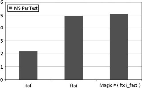
Conversions from float to integer are more costly than from integer to float. On our standard machine, the magic number method, listed as ftoi_fast in the performance harness, showed slightly slower performance than the SSE version compiled by Visual Studio 2008. Figure 7.3 compares several methods for converting from integer to float.

Figure 7.3. Comparison of execution time for different methods for converting from float to integer. Time is in milliseconds.

Vector instructions have a long and distinguished history in the realm of high performance computing. From the early days of vector processing with Cray to the latest SIMD instruction sets like SSE and LRB, vector ops have been the key to speed. SSE uses dedicated hardware registers capable of performing a single instruction on multiple data (SIMD) to achieve parallelism.

Time to rewrite your math library for the N^th time? Well, if it was written sometime in the past decade, it probably already takes advantage of SIMD. If you use the D3DX functions bundled with DirectX, they already take advantage of SSE. However, simply rewriting your math library isn’t going to be your biggest win.

The best place for SSE is going to be when you have a whole algorithm you can SIMDize. When you can stay exclusively in the SSE registers for an extended period, you can often get large performance gains.

The remainder of this section focuses on opportunities for compute wins. For a discussion of SSE’s memory streaming and cache management capabilities, see Chapter 6, “CPU Bound: Memory.”

_ _m128 sseVec = _mm_load_ps( &m_Vector );

#ifndef __WIN32__
#define _align16_ __attribute__((align(16) ))
#else
#define _align16_ __declspec(align(16) )
#endif

__align16__ float m_Vector[4];

__align16__ struct Particles
{
     float m_Position[4];
}

(float*)_mm_malloc( 100 * sizeof(float),16);

_align16_ struct Particle
{
     float position[3];
     float velocity[3];
}

for( int i=0;i<m_NumParticles;i++)
{

     pParticle* pPart = particleArray[i];
     pPartposition.x += pPartvelocity.x;
     pPartposition.y += pPartvelocity.y;
     pPartposition.z += pPartvelocity.z;
}

for( int i=0;i<m_NumParticles;i++ )
{
     pParticle* pPart = particleArray[i];
     AddSSE( pPart->position,
     pPart->velocity,
     pPart->position );
}

void AddSSE( float* vec1, float* vec2, float *out )
{
     __m128 a = _mm_load_ps( vec1 );
     __m128 b = _mm_load_ps( vec2 )
     __m128 c = _mm_add_ps( a, b );
     _mm_store_ps(out, c );
}

_align16_ struct Particle

{
     float posX[100];
     float posY[100];
     float posZ[100];
     float posW[100];
     float velX[100];
     float velY[100];
     float velZ[100];
     float velW[100];
}

for( int i=0;i<m_NumParticles/4;i+=4 )
{
     pParticle* pPart = particleArray[i];
     pPart->position += pPart->velocity;
     __m128 posXvec = _mm_load_ps( pPart->posX[i] );
     __m128 posYvec = _mm_load_ps( pPart->posY[i] );
     __m128 posZvec = _mm_load_ps( pPart->posZ[i] );
     __m128 posWvec = _mm_load_ps( pPart->posW[i] );

     __m128 velXvec = _mm_load_ps( pPart->velX[i] );
     __m128 velYvec = _mm_load_ps( pPart->velY[i] );
     __m128 velZvec = _mm_load_ps( pPart->velZ[i] );
     __m128 velWvec = _mm_load_ps( pPart->velW[i] );

     posXvec = _mm_add_ps( posXvec, vecXvec );
     posYvec = _mm_add_ps( posYvec, vecYvec );
     posZvec = _mm_add_ps( posZvec, vecZvec );
     posWvec = _mm_add_ps( posWvec, vecWvec );

     //remainder of particle update
}

Compilers are smart. You can’t rely on them to do exactly what you want at any given place in the code, but in aggregate, they do a pretty good job. As a programmer, you don’t have the time or motivation to look for a hundred little optimizations in every line of code, but the compiler has plenty of energy for that purpose.

Some developers are very suspicious of their compilers. And indeed, some compilers are worth being suspicious of. As part of your basic profiling work—benchmarking and identifying bottlenecks—you will quickly get a sense of whether you can trust your compiler, because if it isn’t being smart, you’ll catch lots of performance sinks. If you’re using a recent version of a big name compiler, like GCC, Intel, or Visual Studio, it’ll probably do pretty well (even if you have to tweak some options to get there).

Throughout the writing of this book, we’ve included tests to go along with our examples. The ability to write these tests has been challenging due to the fact that it is usually very hard to write wasteful code. Many times, the compiler surprised us by removing code we were hoping to use as our baseline.

No matter where you stand on the issue, it’s difficult to argue that compilers have been doing anything but improving. Newer features, such as Visual Studio’s profile-guided optimization, perform profiles on your executable and compile your program based on the collected data. Take a little time to get to know your compiler, and you will be pleasantly surprised.

int j=0;
int k=0;
for( int i=0;i<100;i++ )
{
     j=10;
     k+=j;
}

k = 1000.0f;

void test()
{
      gCommon +=TestLoopOne();
      gCommon +=TestLoopTwo();
}

float TestLoopOne()
{
      float test1=0.0f;
      for( int i=0;i<1000;i++ )
      {
            test1 += betterRandf();
      }

      return test1;
}

float TestLoopTwo()
{
      float test2=0.0f;

      for( int i=0;i<1000;i++ )
      {
            test2 += betterRandf();

      }

      return test2;
}

CPUs are getting ever faster, but when you run out of computing power, it’s time to optimize. Lookup tables, inlining, dealing with branch prediction, avoiding slow instructions, and SIMD instructions are techniques you can use to enhance the performance of your code. Modern compilers will make the most out of code that doesn’t specifically target performance.

With good profiling techniques, careful design, and iterative improvement, even the worst compute bound application can shine, but don’t forget, computing power has improved much faster than general memory fetching.