Problems of scalability prevent you from seeing continual increases in performance as you increase threading and/or cores. Many multi-threaded algorithms will not continually show an increase in performance as you add threads and cores. Developing an algorithm that will scale indefinitely can be quite daunting. Problems that can scale indefinitely are called “embarrassingly parallel.” Graphics/pixel processing is one such problem, which is why GPUs have been so successful at increasing performance.

For a long time, we pointed to Amdahl’s law when trying to describe one of the typical scalability issues. Amdahl stated that the maximum speedup from parallelization depends on the portion of the task that is serial. The serial portion often occurs where communication between processors exists or when a gathering of information occurs. Using our letter stuffing campaign as an example, serial execution occurs when the letter bin is full and everyone stops adding letters to the bin until the old one is gone and a new bin is in place.

Amdahl’s Law reads:

Where P is the proportion of the program we are speeding up and S is the factor by which we’ve sped that part up. Let’s take a look at what happens if we can take 80% of our program and parallelize it.

As you can see from this graph, ultimately the speed of the app is limited by the part that isn’t parallelized. In other words, the limit to scalability is the serial portion of our app. Of course, in our example, we still made the whole thing X times faster. But that’s assuming that the parallelized part has no serial portions and that the code runs in complete isolation from the rest of the system until it’s synchronized.

In 1988, Gustafson came up with his own law, which offers another solution to the calculation of predicting scalability.

Gustafson’s Law reads:

Where a(n) is the serial function and p is the number of processors. Gustafson states that the significance of the serial portion becomes less a contributing factor as n approaches infinity. In other words, according to Gustafson, if the size of the job of the parallel algorithm can grow to be larger and larger, so can our returns of being parallel since the serial part does not necessarily grow linearly with the parallel part.

For an example of how Gustafson’s Law plays out, let’s look at image processing. There is a serial part (loading and unloading the buffers holding the image) and a parallel part (running the processing kernel on each pixel). The more complex the kernel, the bigger the speedup from parallelization because it will overshadow the cost of copying data into/out of the buffer. In this example, increasing the size of the image can improve performance gain, as long as your processing time per byte is greater than your transfer time.

To add to the confusion, Shi suggests that there is, in fact, one law and the two equations are actually equal (Shi, 1996). Shi states that determining the concept of a serial percentage of a program is misleading and that Gustafson’s definition of p is different than Amdahl’s.

Computer scientists continue to cite and dispute the methods for predicting parallel performance increase. But there is one thing they won’t dispute: Serial execution in a parallel algorithm is bad for performance. When designing a parallel algorithm, consider what elements of your algorithm will cause serial execution and do your best to reduce or remove them.

In a perfect world, we would be able to write programs that could be entirely parallelized with no serial portion at all. But practically, we run into a major issue related to our desire for our program to execute correctly and in a reliable and consistent manner. This limiting factor is called contention. Contention occurs when one or more threads attempt to access the same resource at the same time.

Imagine each resource as an intersection. Cars (threads) pass through it in several directions at once. If cars go through with no regulation, then eventually there will be a wreck, either a literal crash or incorrect program behavior.

There are many ways to tackle this problem. They vary in complexity, performance, and effectiveness.

The simplest solution is to put up stop signs. Threads use the resource on a first-come, first-served basis. You can implement this by using a mutex. This approach requires each thread to lock the mutex while they’re using the resource, and you’re set. You’ll often see this approach used to quickly make a subsystem thread-safe—for instance, a memory manager will often have a global mutex.

Another option is to replace the intersection with separate, nonintersecting roads. For instance, we might give each thread its own local heap, instead of making them contend over a single global heap. But in some cases, this isn’t feasible. For instance, memory usage by threads might be so great that there isn’t enough to reserve for each thread’s heap. Or the shared resource might need to be common between all threads in order for correct program execution, like a draw queue.

Even though a resource might need to be shared, it doesn’t need to be exactly in sync all the time. For instance, the draw queue might only need to be double buffered rather than shared, reducing the number of potential contentions from hundreds a frame to one.

A third option is to look for more efficient synchronization. In the context of the intersection, this is like installing stoplights and allowing turns on red. Sometimes, you can break up a single resource into multiple parts that can be accessed independently, for example, do finer-grained synchronization. Other times, you can use hardware support to make synchronization operations faster. In yet other cases, it may be possible to remove extraneous synchronization checks.

Synchronization primitives (mutexes, locks, semaphores, atomic operations, etc.) are essential for correct functioning. But each one holds the possibility for your threads to fall back into a serial mode and lose all the performance gains you get from concurrency. Serial operation, as we noted in the previous section, is a major limiter for performance of multi-threaded implementations.

Balancing workload is the final third of the thread performance picture. Just as the whole computer must have a balanced workload for maximum efficiency, your various computing tasks need to be balanced among the different hardware elements that can run them. It’s no good having a multi-threaded application that uses one core completely and leaves the rest untouched.

We already have a powerful set of techniques for measuring this, which are the same profiling techniques we have been discussing throughout this book. Look at the CPU utilization of the cores on your target system, and if they are uneven, determine what factor is preventing them all from being used evenly. Likely causes are starvation (not enough work to keep them all busy, or an artificial limit preventing work from being allocated properly) or serialization (for example, dependencies between tasks that force them to be executed in order rather than in parallel).

The rest of this chapter goes into more detail on strategies for keeping workloads balanced.

A critical section and mutex have similar functionality with different implementations and performance implications. A critical section is a userspace anonymous mutex, and a Win32 mutex is an interprocess named mutex. There can be any number of either critical sections or mutexes. The functionality provides the easy ability to place an enter-and-leave call before and after a section of code that you want to protect from access by more than one thread or (in the case of the Win32 Mutex) process at a time.

Imagine two lakes connected by channels wide enough for only one boat. If any boats (threads) want to navigate to the other lake, they must first determine if the channel they want to use is empty before entering. This channel, where only one boat can fit at any time, is similar to a critical section or a mutex.

When a thread enters a critical section or takes a mutex, any other thread wishing to enter the critical section or take the mutex will contend for that space and block, until the occupying thread leaves the section or releases the mutex. Contention, as noted previously, is a cause of serial operation and a limiter of performance increases.

In Windows, the difference between a critical section and the mutex is the level at which the synchronization primitive is visible. The critical section implementation is only visible within an application; the mutex implementation is visible between applications as well. A mutex will be slower on average than a critical section, because it must deal with more complex scenarios. In most cases, you only need to synchronize between threads in the same application, so the critical section will be the most commonly used option.

The critical section and mutex, in Windows, share a similar interface. A critical section will use the syntax of Enter and Leave to specify areas of code where only one processor can enter at any given moment. A mutex will use a wait-function to enter the protected code and a ReleaseMutex call to exit the protected call.

Critical sections and mutexes are powerful and easy to use; unfortunately, they are also easy to abuse. For performance considerations, developers should not think of these two synchronization objects simply as a means for preventing multi-threading problems. Since contention is expensive, and noncontention is not, developers should create their algorithms with the goal of naturally reducing contention. If you design this way, you can use critical sections and mutexes as a failsafe in the unlikely event that two or more threads attempt to enter the same area at the same time. Reducing contention as much as possible is ideal.

Windows has a traditional semaphore implementation. A windows semaphore object uses ReleaseSemaphone to increment the semaphore and a WaitFor*Object() to decrement it.

An event in Windows is a binary semaphore. So instead of being able to increment an event, it only has two states: signaled and nonsignaled. They are marked as signaled by using SetEvent().

WaitForSingleObject, supplied with a handle to an appropriate object, and WaitForMultipleObjects, supplied with an array of handles, are two calls you can use to block these objects. For example, you can call WaitForSingleObject on an event handle to create an OS implemented blocking system to keep a thread waiting efficiently for another thread to signal the event. The wait function also has a parameter for setting a time-out interval. This time-out can be set to INFINITE, which implies that the function will wait indefinitely to control the semaphore, mutex, or event, or you can set a millisecond value that specifies a wait time before “giving up” on the wait and moving on.

HANDLE mutex = CreateMutex( NULL, FALSE, NULL );

DWORD dwWaitResult = WaitForSingleObject( mutex , INFINITE );

If( dwWaitResult )
{

    //critical code
    ReleaseMutex( mutex );
}

In a typical race, the winner is the person who arrives first. In a race condition, the winner may be the thread that gets to a memory address last.

A race condition creates incorrect data due to unexpected interactions between threads. The classic example is two threads trying to increment the same variable. The interaction should go something like this:

If the value started at 1, now we have 3. But depending on the order of execution, the following could occur:

In which case, we end up with 2. Whoever writes his invalid data last has won the race and broken the program.

A race condition creates incorrect results due to the issue of order; false sharing describes an issue with one or more cores using a memory address at the same time (or very near to the same time). It cannot happen in single core execution for reasons that will become clear shortly.

From the earlier chapter on memory, you should understand that memory utilizes a hierarchy of registers, caches, and DRAM. As the cache hierarchy transfers data, there is the potential for data to get out of sync. For instance, if one core reads some memory into cache right before another core writes to the same memory, there is the potential for the first core to have old values in its cache. When two or more cores share a cache line, the memory subsystem may force serial updates of the shared line to maintain data integrity. This serialization, known as sharing, creates an overhead that the program can do without. Figure 13.1 further explains the process in steps.

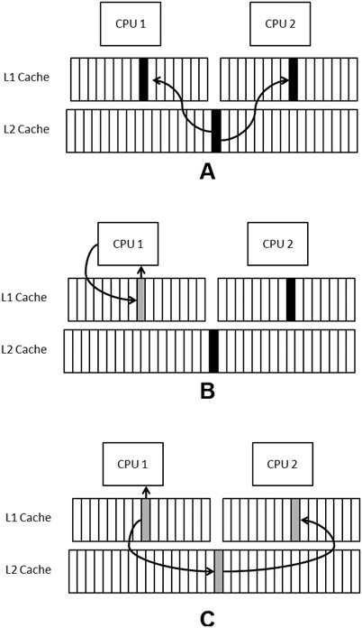
Figure 13.1. A shows the same data being loaded into two CPU’s caches. B shows CPU 1 writing to the shared data. C shows corrective action being taken by the system to propagate the change to CPU 2’s cache.

Consider two cores, 1 and 2, that read the same cache line from DRAM into the L2 cache and L1 cache (A). So far, coherency is maintained. If core 1 changes a value in the cache line, a coherency issue occurs (B). This type of issue is common for a single thread, the discrepancy of the value in core 1’s register is temporary and eventually the value of the register will copy to the cache and back to the DRAM. In this case, however, there is another discrepancy that exists between the register in core 1 and the register in core 2. This discrepancy is unacceptable and could lead to inaccuracies.

The hardware solves this problem the only way it can—by blocking core 2 from proceeding and forcing an update to occur that ensures the values in core 2’s register match the L1 caches, the L2 cache, and core 2’s registers. This comes at a cost of the update and time lost for the synchronization to occur. (When a CPU does this, it will also drop any predicatively executed results so that code runs consistently.) This update process is known as sharing.

False sharing is similar, but a bit more obtuse. Since the synchronization occurs when sharing cache lines, this type of synchronization can occur when core 1 and core 2 are working with completely different variables. The usual suspects are member variables or global variables being acted upon by two different cores at the same time.

In the worst case, false sharing can result in every core in the system running in serial, since each updates a cache line in turn and then blocks until every other core gets a chance to process the update. This results in a ping-pong effect because each processor runs in a serial mode updating the other.

Sharing of the same variable should be avoided; it is likely also a race condition. While false sharing will not result in a race condition, it still incurs the performance penalty of sharing. In the case of false sharing, the solution is easy: ensure that variables that are frequently updated by different threads are not on the same cache line.

struct vertex
{
   float xyz[3]; //data 1
   float tutv[2];//data 2
};

vertex triList[N];

Let’s use a vertex as an example to discuss the possible solutions. Let’s assume that core 1 is working with data 1 and core 2 with data 2. We could pad the shared variables so they aren’t on the same cache line, and although this would work, we have greatly bloated the size of the array.

We could reorganize the implementation to have core 1 operate on all even vertices and core 2 operate on the odd. This case will work well if the vertex is 64-byte aligned and 64 bytes in size (which is actually a popular vertex size). If it is close, padding by four bytes or so is probably an acceptable trade-off.

A better solution would be to convert the array of structures to a structure of arrays. The data is now separated and each core can access its data linearly, as opposed to periodically, a requirement of the prior structure.

struct vertices
{
   float xyz[3][N];   // Core 1
   float tutv[2][N]; // Core 2
};

vertices triList;

False sharing is not ideal; however, it’s not as bad as it once was. Cores on the same chip often have shared caches, which removes the need for them to synchronize by writing all the way out to DRAM.

A deadlock occurs when two or more threads are mutually blocking. A deadlock is similar to a stalemate in chess—nothing wrong occurred per se, but the game is over and no one can move. Deadlocks can occur for many reasons, but typically, they are the result of faulty logic causing interdependent synchronization objects.

Let’s start with a simple example. Let’s take two threads, X and Y, and two critical sections, CSa and CSb. A deadlock would occur if the following order of events were to occur:

Thread X waits indefinitely for Y’s release of CSb, and thread Y waits indefinitely for X’s release of CSa—they will wait forever. Deadlocks aren’t performance concerns that you can optimize; you just need to remove them.

Deadlock occurrences are measureable statistically, meaning they can occur on a spectrum of having a high-to-low probability. A deadlock that has a one-in-a-million chance to occur is very hard to debug and chances are that there is a lot of shipped software with deadlocks in this probability. To combat this problem, there are tools that can perform a statistical analysis of your code and report where deadlocks may occur. One such program is Intel’s Thread checker.

The previous example, if performed in a different order, would not have triggered a deadlock. If the OS created context switches in the following order, the code would proceed:

Resource contention can be an issue, but it’s usually possible to avoid it with good design. For instance, if you are going to be doing a lot of disk IO, you might want to have a worker thread that services disk requests instead of having each thread do its own IO and potentially overloading the disk. Or if two threads are going to access the same section of memory frequently, they might benefit from having their own copies of the data.

If you’re writing useful programs, you’ll have to deal with contention issues. In the last section, we talked about some situations where contention comes up and some ways to deal with it. But what are common reasons for contention to be needed?

Hidden locks can be a big performance hog, because they typically aren’t added with performance in mind. Third-party code can sometimes have synchronization primitives in it that cause problems. For instance, a memory allocator might have a lock to access a shared heap. If you have threads that are frequently allocating or freeing memory, this can completely kill performance, effectively reducing the threads to serial execution. The hardware can sometimes enforce synchronization, too, for instance if two threads are trying to write to the same area in memory.

At a basic level, you can spot threading performance issues by looking for lost time, time spent idle or waiting on synchronization primitives. If you see that 80% of your thread’s time is spent trying to acquire locks, you know that something is wrong. Make sure that you have a profiler that supports multiple threads!

Look for normal API calls that sometimes take much longer than expected, as this is a sign of hidden locks or other forms of contention. If printf starts taking up 50% of your time when you add a second thread that prints, you should check whether it has a lock in it.

There are a few considerations to keep in mind when measuring threading performance. Look out for “heisenbugs,” which are problems that disappear or appear when you try to observe them. Sometimes, the profiler can alter execution sufficiently to change your performance bottlenecks. Make sure that you test with a real workload; threading is indeterminate, so your numbers may change dramatically, depending on the situation.

Looking at it from a positive perspective, when you add threading, you should be measuring overall time for your benchmark. It’s helpful to be able to execute in both a single-thread or multi-thread mode; then you can quickly do A/B comparisons to see where you’re at performance wise. Sometimes, all that’s needed for this is to force CPU affinity so that the program only runs on a single core. Additionally, you should be looking at the utilization of the resources that you intend to be using (for example, the other cores). When running with multiple threads, you should see much more even distribution of load.

Setting CPU affinity can also help identify some race conditions. If you force everything to run on one core, it has to be run in serial. Doing this lets you remove simultaneous access of data as a potential cause of problems.

In the case of using a thread to manage a slow resource (like disk access), you probably won’t see a spike in utilization. Instead, you’ll see a reduction in latency spikes—i.e., more regular and even frame times.

First, look at your threading approach from a high level. Amdahl’s Law is useful here; you can determine some theoretical limits on performance. Be aware that Amdahl’s Law requires full knowledge of the system to be entirely accurate. If you only model part of the system with it, you may not be properly estimating available performance. For instance, sometimes you can get super-linear speedups because the hardware is better utilized by multiple threads.

Then you can use the usual process. Grab a multi-thread-capable profiler, identify the biggest performance loss, and fix it. Measure and repeat.

The best tactic for optimizing concurrent applications is removing sources of contention—attempts to lock mutexes, semaphores, etc. You must be careful that you don’t sacrifice the correct functioning of your program. From there, it’s very similar to optimizing a serial application.

There are some new tactics you can use. Try to keep high-use resources thread-local. If your thread is going to be allocating a lot of memory, give it its own local buffer of memory to use, so it doesn’t have to hit the global heap all the time.

Depending on your hardware, you might be able to use so-called lockless algorithms, which can be much more efficient because they bring the granularity of synchronization down to single elements in a data structure. They require specific hardware support, so you have to be careful not to rely on functionality that only some users will have.

Finally, try to defer synchronization, if synchronization is costly. For instance, let a thread buffer several work elements before it merges them into the final result set. If you are doing lots of little tasks, this can save significant amounts of overhead.

The simplest (incorrect) implementation of the ReadWriter would be to have a shared variable that threads could access. A writer thread could write to a variable and then a reader thread would read the value. Writing variables is not guaranteed to be atomic, so if one thread is writing to the memory, the reading thread may perform a read on a partially written value. This partial update is known as tearing, an occurrence you must protect against.

If you were to make the shared variable’s reading and writing atomic, say by surrounding the shared variable with a critical section, or by using atomic operations (for instance, InterlockedIncrement on Win32), then the transaction would be safe; however, this is not optimal. In the best case, the two threads would behave serially, with a ping-pong-like transaction involving one thread waiting for the other to exit the critical section.

You might assume that two cores running at 50% give a similar performance to one core running at 100%, but that is not the case. Switching from one thread to another involves overhead in both hardware and in the OS. So in this implementation, two threads taking turns in lockstep is not as fast as one thread running without the overhead of thread switching.

In Figure 13.3, you can see that while one thread is running, the other is waiting—each thread is running in lockstep. In the multi-thread visualization, each core is spending nearly as much time waiting as it does running, and each switch comes at a cost that limits the overall utilization.

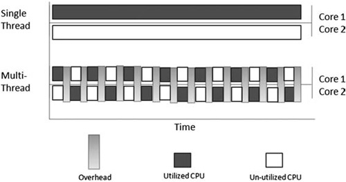
Figure 13.3. Visualization showing how a single-threaded implementation with no overhead achieves better utilization than a dual-threaded implementation that causes costly overhead due to the switching that occurs when two threads execute in lockstep.

How bad is the overhead of switching cores? Well, let’s run an experiment to find out.

We are able to create this lock-step behavior using the PerformanceHarness example threading/writeReader and defining THREADSTREAM to 0 at the top of the file.

Running this code on our test machines and using Intel’s Thread Profiler yields statistics about the active time for the two threads. By examining a 500-millisecond section of execution during the writing and reading, we find that thread 1 is active, meaning not in a wait state, for about 370 milliseconds and thread 2 is active for about 300 milliseconds. This yields a combined total of 670 milliseconds or 67% of the total 1,000 milliseconds possible (2 threads × 500 milliseconds). Of the 670 active milliseconds, 315 milliseconds are spent in serial operations attributable to the critical sections used to implement the synchronization. This inefficiency leads us with only 355 (670-315) milliseconds of real processing. So to summarize, we are only utilizing the processor for 35.5% of the total that is theoretically possible for this time span.

Running this test 10 times provides an average time that we can use for comparison with later implementations. When tested, the benchmarks average for 10 tests is around 2.422 seconds. It should also be noted that the number of contentions is so high, that the Thread Profiler takes quite some time to visualize them all.

For the next optimization, let’s increase the single variable to an array, similar to the visualization in Figure 13.4. At each array point, we will have a space for a value and a synchronization primitive.

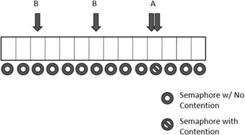
Figure 13.4. Contentions could dramatically be reduced by switching from a single variable to an array. In case A, a contention occurs. In case B, a contention does not.

You can re-create this example by defining the preprocessor value THREADSTREAM to 1. This implementation has some significant advantages over the single variable approach in the previous attempt. The likelihood of experiencing a contention is significantly reduced since, instead of a guaranteed contention, the program has the potential for contention, meaning that it doesn’t always contend. The more you increase the ARRAY_SIZE defined value, the less likely you are to contend.

Intel’s thread profiler confirms this approach and the utilization is high. Using the previous implementation, both threads are nearly 100% utilized. We are able to move through 1,000,000 integers in roughly 106 milliseconds, which is a 2,179% performance increase.

Earlier in this book, we discussed the three levels of optimization: system, application, and micro. Those lessons transfer well to optimizing our algorithm. By reducing the contentions, we have increased the utilization, which is a step in the right direction.

But a high utilization doesn’t automatically mean that we have the fastest algorithm. If you sit behind your desk all day at work and search the Internet, you might be busy, but your productivity is horrible. To optimize, we must have both high utilization and efficient processing. That leads us to our next optimization.

For our final implementation, we will build on the array approach by reducing the number of critical section enter-and-leave calls by maintaining a mutex for each section of the array. Figure 13.5 shows the approach.

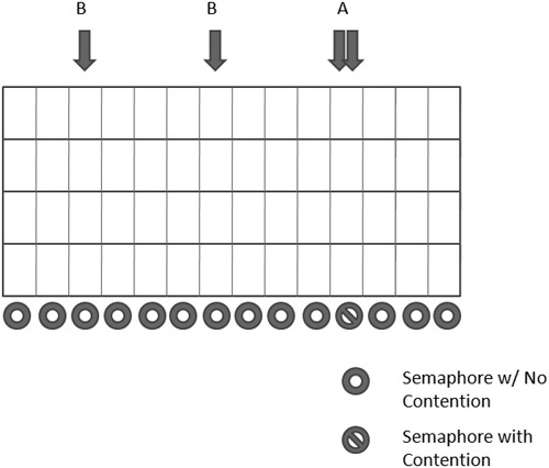
Figure 13.5. Notice that no contention occurs except at point A, where two threads try to access the same data at the same time.

In the array implementation, we have an enter-and-leave call for every read or write. By using an array-of-arrays instead of one big array, we can have a lock per row. This reduces the overhead of enter-and-leave calls and uses more of our processor for processing data. You can re-create this example by setting the preprocessor define THREADSTREAM equal to 2.

Utilization is great, and now the processing is more efficient and takes advantage of the CPU’s ability to step quickly through linear memory. Our implementation is now running in 9.9 milliseconds, an appreciable performance gain.

For a test, we implemented a single-threaded version of the reader writer and compared it to the multi-threaded version. The results are not incredibly impressive; the single-threaded implementation achieves nearly 11.5 milliseconds, which begs the question of why so much work was done for such a small increase and the potential for such bad performance.

The answer lies in scaling. The delta between these two implementations improves performance as we increase the number of integers. By upping the ITERATION to 10,000,000, the threaded version becomes nearly twice as fast in total execution time instead of just slightly ahead. By increasing the thread count to four, the average time moves to 6.9 milliseconds.

Conversely, increasing the thread count to six reduces performance to 9.1 milliseconds. Why? Executing more intensive threads than cores will create over-utilization, a term that defines a condition in which we are using more software threads than the number of simultaneous threads in hardware. There are many references that suggest the optimal thread ratio is 1:1 cores to threads, but there are very few examples of why.

We found that the biggest contributor to this is not overhead caused by having too many threads. We do not believe that the OS will increase context switches by shortening time slices and the processor doesn’t manage threads, so it has no say in the matter as well. (Even in the case of Hyper-Threading, the CPU doesn’t schedule. It just allows two threads at a time to run on the same core.)

A key issue is synchronization. Synchronization is slower when there isn’t a one-to-one relationship of thread to hardware. Four threads can synchronize nearly instantly on a four-core machine. When we run six threads on a four-core machine, only four can synchronize concurrently. The remaining two will require a thread context switch from the other threads. The serialization of these threads can be significant, especially if the OS is switching to other threads in-between the serialization.

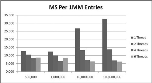
If synchronization is the issue, then algorithms with larger concurrency-to-synchronization ratios should see less of a performance problem. This data is presented in Figure 13.6.

Figure 13.6. Elapsed time, normalized for 1,000,000 entries, for varying numbers of entries and threads. On our four-core test system, four threads gave the consistently best performance.

Lastly, the source code for these tests provides us more information on sharing, balancing, and synchronization primitives.

Several variables in the source have the _ _declspec(align(64)) preprocessor directive (not cross platform). This is because the variables nearby have the possibility to incur performance hits due to false sharing. By forcing 64-byte alignement, the variable will have its own cache line, eliminating any opportunity for false sharing.

To experiment with balancing, try allocating an uneven number of readers and writers. By default, the program allocates one reader for every writer.

Finally, there were many efforts taken to increase the performance of synchronization primitives. Events provided a faster implementation for signaling from one thread to another. In this algorithm, events were much faster than implementing spinlocks with volatile Boolean variables.