8
MISCELLANEOUS UML DIAGRAMS

This chapter finishes up the book’s discussion of UML by describing five additional diagrams that are useful for UML documentation: component, package, deployment, composite structure, and statechart diagrams.

8.1 Component Diagrams

UML uses component diagrams to encapsulate reusable components such as libraries and frameworks. Though components are generally larger and have more responsibilities than classes, they support much of the same functionality as classes, including:

• Generalization and association with other classes and components
• Operations
• Interfaces

UML defines components using a rectangle with the «component» stereo­type (see Figure 8-1). Some users (and CASE tools) also use the stereotype «subsystem» to denote components.

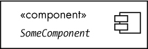
Figure 8-1: A UML component

Components use interfaces (or protocols) to encourage encapsulation and loose coupling. This improves the usability of a component by making its design independent of external objects. The component and the rest of the system communicate via two types of predefined interfaces: provided and required. A provided interface is one that the component provides and that external code can use. A required interface must be provided for the component by external code. This could be an external function that the component invokes.

As you would expect from UML by now, there’s more than one way to draw components: using stereotype notation (of which there are two versions) or ball and socket notation.

The most compact way to represent a UML component with interfaces is probably the simple form of stereotype notation shown in Figure 8-2, which lists the interfaces inside the component.

Figure 8-2: A simple form of stereotype notation

Figure 8-3 shows a more complete (though bulkier) version of stereotype notation with individual interface objects in the diagram. This option is better when you want to list the individual attributes of the interfaces.

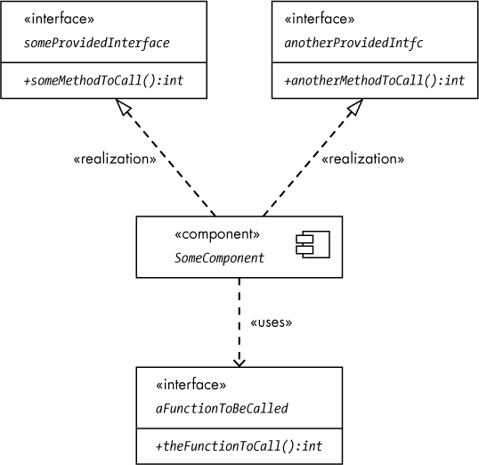
Figure 8-3: A more complete form of stereotype notation

Ball and socket notation provides an alternative to the stereotype notation, using a circle icon (the ball) to represent a provided interface and a half-circle (the socket) to represent required interfaces (see Figure 8-4).

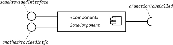
Figure 8-4: Ball and socket notation

The nice thing about ball and socket notation is that connecting components can be visually appealing (see Figure 8-5).

Figure 8-5: Connecting two ball and socket components

As you can see, the required interface of component1 connects nicely with the provided interface of component2 in this diagram. But while ball and socket notation can be more compact and attractive than the stereotype notation, it doesn’t scale well beyond a few interfaces. As you add more provided and required interfaces, the stereotyped notation is often a better solution.

8.2 Package Diagrams

A UML package is a container for other UML items (including other packages). A UML package is the equivalent of a subdirectory in a filesystem, a namespace in C++ and C#, or packages in Java and Swift. To define a package in UML, you use a file folder icon with the package name attached (see Figure 8-6).

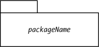
Figure 8-6: A UML package

For a more concrete example, let’s return to the pool monitor application. One useful package might be sensors, to contain classes/objects associated with, say, pH and salinity sensors. Figure 8-7 shows what this package might look like in UML. The + prefix on the phSensors and saltSensor objects indicates that these are public objects accessible outside the package.¹

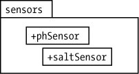
Figure 8-7: The sensors package

To reference (public) objects outside of a package, you use a name of the form packageName::objectName. For example, outside the sensors package you would use sensors::pHSensor and sensors::saltSensor to access the internal objects. If you have one package nested inside another, you could access objects in the innermost package using a sequence like outsidePackage::internalPackage::object. For example, suppose you have two nuclear power channels named NP and NPP (from the use case examples in Chapter 4). You could create a package named instruments to hold the two packages NP and NPP. The NP and NPP packages could contain the objects directly associated with the NP and NPP instruments (see Figure 8-8).

Figure 8-8: Nested packages

Note that the NP and NPP packages both contain functions named calibrate() and pctPwr(). There is no ambiguity about which function you’re calling because outside these individual packages you have to use qualified names to access these functions. For example, outside the instruments package you’d have to use names like instruments::NP::calibrate and instruments::NPP::calibrate so that there is no confusion.

8.3 Deployment Diagrams

Deployment diagrams present a physical view of a system. Physical objects include PCs, peripherals like printers and scanners, servers, plug-in interface boards, and displays.

To represent physical objects, UML uses nodes, a 3D box image. Inside the box you place the stereotype «device» plus the name of the node. Figure 8-9 provides a simple example from the DAQ data acquisition system. It shows a host PC connected to a DAQ_IF and a Plantation Productions’ PPDIO96 96-channel digital I/O board.

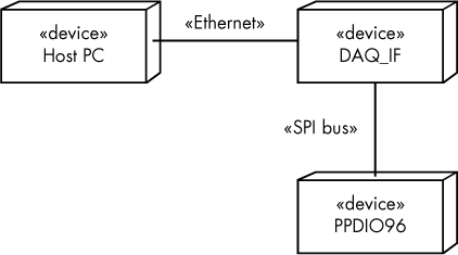
Figure 8-9: A deployment diagram

One thing missing from this figure is the actual software installed on the system. In this system, there are likely to be at least two application programs running: a program running on the host PC that communicates with the DAQ_IF module (let’s call it daqtest.exe) and the firmware program (frmwr.hex) running on the DAQ_IF board (which is likely the true software system the deployment diagram describes). Figure 8-10 shows an expanded version with small icons denoting the software installed on the machines. Deployment diagrams use the stereotype «artifact» to denote binary machine code.

Figure 8-10: An expanded deployment diagram

Note that the PPDIO96 board is directly controlled by the DAQ_IF board: there is no CPU on the PPDIO96 board and, therefore, there is no software loaded onto the PPDIO96.

There is actually quite a bit more to deployment diagrams, but this discussion will suffice for those we’ll need in this book. If you’re interested, see “For More Information” on page 165 for references that explain deployment diagrams in more detail.

8.4 Composite Structure Diagrams

In some instances, class and sequence diagrams cannot accurately depict the relationships and actions between components in some classes. Consider Figure 8-11, which illustrates a class for the PPDIO96.

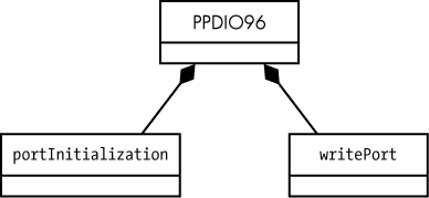
Figure 8-11: PPDIO96 class composition

This class composition diagram tells us that the PPDIO96 class contains (is composed of) two subclasses: portInitialization and writePort. What it does not tell us is how these two subclasses of PPDIO96 interact with each other. For example, when you initialize a port via the portInitialization class, perhaps the portInitialization class also invokes a method in writePort to initialize that port with some default value (such as 0). The bare class diagrams don’t show this, nor should they. Having portIntialization write a default value via a writePort invocation is probably only one of many different operations that could arise within PPDIO96. Any attempt to show allowed and possible internal communications within PPDIO96 would produce a very messy, illegible diagram.

Composite structure diagrams provide a solution by focusing only on those communication links of interest (it could be just one communication link, or a few, but generally not so many that the diagram becomes incomprehensible).

A first (but problematic) attempt at a composite structure diagram is shown in Figure 8-12.

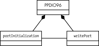
Figure 8-12: Attempted composite structure diagram

The problem with this diagram is that it doesn’t explicitly state which writePort object portInitialization is communicating with. Remember, classes are just generic types, whereas the actual communication takes place between explicitly instantiated objects. In an actual system the intent of Figure 8-12 is probably better conveyed by Figure 8-13.

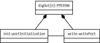
Figure 8-13: Instantiated composite structure diagram

However, neither Figure 8-12 nor Figure 8-13 implies that the portInitialization and writePort instantiated objects belong specifically to the PPDIO96 object. For example, if there are two sets of PPDIO96, portInitialization, and writePort objects, the topology in Figure 8-14 is perfectly valid based on the class diagram in Figure 8-12.

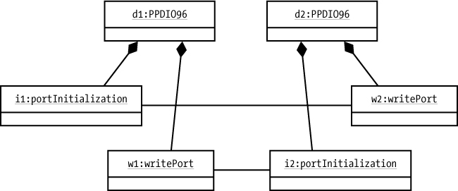
Figure 8-14: Weird, but legal, communication links

In this example, i1 (which belongs to object d1) calls w2 (which belongs to object d2) to write the digital value to its port; i2 (which belongs to d2) calls w1 to write its initial value to its port. This probably isn’t what the original designer had in mind, even though the generic composition structure diagram in Figure 8-12 technically allows it. Although any reasonable programmer would immediately realize that i1 should be invoking w1 and i2 should be invoking w2, the composite structure diagram doesn’t make this clear. Obviously, we want to eliminate as much ambiguity as possible in our designs.

To correct this shortcoming, UML 2.0 provides (true) composite structure diagrams that incorporate the member attributes directly within the encapsulating class diagram, as shown in Figure 8-15.

Figure 8-15: Composite structure diagram

This diagram makes it clear that an instantiated object of PPDIO96 will constrain the communication between the portInitialization and writePort classes to objects associated with that same instance.

The small squares on the sides of the portInitialization and writePort are ports. This term is unrelated to the writePort object or hardware ports on the PPDIO96 in general; this is a UML concept referring to an interaction point between two objects in UML. Ports can appear in composite structure diagrams and in component diagrams (see “Component Diagrams” on page 155) to specify required or provided interfaces to an object. In Figure 8-15 the port on the portInitialization side is (probably) a required interface and the port on the writePort side of the connection is (probably) a provided interface.

In Figure 8-15 the ports are anonymous. However, in many diagrams (particularly where you are listing the interfaces to a system) you can attach names to the ports (see Figure 8-16).

Figure 8-16: Named ports

You can also use the ball and socket notation to indicate which side of a communication link is the provider and which side has the required interface (remember, the socket side denotes the required interface; the ball side denotes the provided interface). You can even name the communication link if you so desire (see Figure 8-17). A typical communication link takes the form name:type where name is a unique name (within the component) and type is the type of the communication link.

Figure 8-17: Indicating provided and required interfaces

8.5 Statechart Diagrams

UML statechart (or state machine) diagrams are very similar to activity diagrams in that they show the flow of control through a system. The main difference is that a statechart diagram simply shows the various states possible for a system and how the system transitions from one state to the next.

Statechart diagrams do not introduce any new diagramming symbols; they use existing elements from activity diagrams—specifically the start state, end state, state transitions, state symbols, and (optionally) decision symbols, as shown in Figure 8-18.

Figure 8-18: Elements of a statechart diagram

A given statechart diagram will have exactly one start state symbol; this is where activity begins. The state symbols in a statechart diagram always have an associated state name (which, obviously, indicates the current state). A statechart diagram can have more than one end state symbol, which is a special state that marks the end of activity (entry into any end state symbol stops the state machine). Transition arrows show the flow between states in the machine (see Figure 8-19).

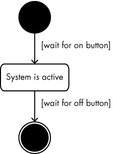
Figure 8-19: A simple statechart diagram

Transitions usually occur in response to some external events, or triggers, in the system. Triggers are stimuli that cause the transition from one state to another in the system. You attach guard conditions to a transition, as shown in Figure 8-19, to indicate the trigger that causes the transition to take place.

Transition arrows have a head and a tail. When activity occurs in a statechart diagram, transitions always occur from the state attached to the arrow tail to the state pointed at by the arrowhead.

If you are in a particular state and some event occurs for which there is no transition out of that state, the state machine ignores that event.² For example, in Figure 8-19, if you’re already in the “System is active” state and an on button event occurs, the system remains in the “System is active” state.

If two transitions out of a state have the same guard condition, then the state machine is nondeterministic. This means that the choice of transition arrow is arbitrary (and could be randomly chosen). Nondeterminism is a bad thing in UML statechart diagrams, as it introduces ambiguity. When creating UML statechart diagrams, you should always strive to keep them deterministic by ensuring that the transitions all have mutually exclusive guard conditions. In theory, you should have exactly one exiting transition from a state for every possible event that could occur; however, most system designers assume that, as mentioned before, if an event occurs for which there is no exit transition, then the state ignores that event.

It is possible to have a transition from one state to another without a guard condition attached; this implies that the system can arbitrarily move from the first state (at the transition’s tail) to the second state (at the head). This is useful when you’re using decision symbols in a state machine (see Figure 8-20). Decision symbols aren’t necessary in a statechart diagram—just as for activity diagrams, you could have multiple transitions directly out of a state (such as the “System is active” state in Figure 8-20)—but you can sometimes clean up your diagrams by using them.

Figure 8-20: A decision symbol in a statechart

8.6 More UML

As has been a constant theme, this is but a brief introduction to UML. There are more diagrams and other features, such as the Object Constraint Language (OCL), that this book won’t use, so this chapter doesn’t discuss them. However, if you’re interested in using UML to document your software projects, you should spend more time learning about it. See the next section for recommended reading.

8.7 For More Information

Bremer, Michael. The User Manual Manual: How to Research, Write, Test, Edit, and Produce a Software Manual. Grass Valley, CA: UnTechnical Press, 1999. A sample chapter is available at http://www.untechnicalpress.com/Downloads/UMM%20sample%20doc.pdf.

Larman, Craig. Applying UML and Patterns: An Introduction to Object-Oriented Analysis and Design and Iterative Development. 3rd ed. Upper Saddle River, NJ: Prentice Hall, 2004.

Miles, Russ, and Kim Hamilton. Learning UML 2.0: A Pragmatic Introduction to UML. Sebastopol, CA: O’Reilly Media, 2003.

Pender, Tom. UML Bible. Indianapolis: Wiley, 2003.

Pilone, Dan, and Neil Pitman. UML 2.0 in a Nutshell: A Desktop Quick Reference. 2nd ed. Sebastopol, CA: O’Reilly Media, 2005.

Roff, Jason T. UML: A Beginner’s Guide. Berkeley, CA: McGraw-Hill Education, 2003.

Tutorials Point. “UML Tutorial.” https://www.tutorialspoint.com/uml/.