
Nanomagnetic Materials
One of the guiding principles of nanotechnology is the observed changes in properties between bulk and nanoscale materials. Perhaps the best example of this principle is observed from magnetic nanomaterials, wherein magnetic properties can be altered drastically with the size of the material. Chapter 5 discusses the origin of magnetic property changes in nanoscale materials, while also discussing synthetic techniques and emerging applications.
Keywords
Nanoscale magnetic properties; magnetic fluids; giant magnetoresistance
5.1 Types of Nanomagnetic Materials [1]
5.1.1 Artificial and Natural Nanomagnetic Materials
Magnetic nanomaterials research and application can be traced back to the 1950s. Quasi-zero-dimensional magnetic nanoparticles were among the first group to be applied [2] and, principally, used in the following three areas. The first is trichoplusia technology for magnetic domain observation. The sample surface is coated with colloidal suspensions comprising iron magnetic powder that is thin. The bulk magnetic field at domain walls has the concentration of the magnetic powder here, which depicted the surface structure of the magnetic domain or the surface trajectory of domain wall. The second is the preparation of single-domain magnetic powder materials. Because the magnetization reversal process of single-domain particles is essentially the magnetic domain rotation without a motion process of the domain wall, the coercivity can be improved significantly. And the third is magnetic fluid for magnetic sealing, for example magnetic seal for spacesuit helmets in the 1960s. The superparamagnetic feature of nanoparticles is applied here. Astronaut helmets are sealed with nanomagnetic materials (magnetic fluid), and this was one of the earliest significant applications.
In 1988, amorphous FeSiB was annealed and doped with Cu and Nb control crystals to develop a novel nanocrystalline soft magnetic material. In the same year, magnetic multilayers were discovered with a giant magnetoresistance (GMR) effect, thus producing a novel discipline: spin electronics.
Theoretical research in 1993 demonstrated that the composition of soft and hard nanoscale magnetic particles could combine the advantages of higher Ms value of soft magnets with the higher Hc value of hard magnets, which could produce a novel nanohard magnetic material with magnetic energy levels twice that of the current top NdFeB material. Research in the twenty-first century has been very active regarding the use of template-based growth of one-dimensional magnetic nanowires, including materials such as single metal, alloy, compounds, multilayer materials, and composite materials, with potential applications ranging from storage medium to cell separation.
Nanomagnetic materials are mainly artificial. However, research has also noted that natural nanomagnetic particles might be found contained within many organisms, such as magnetic bacteria, pigeons, dolphins, stone turtles, bees, the human brain, and so on. In 1975, a string of magnetic nanoparticles was found within the body of magnetic bacteria. As mentioned in Chapter 1, magnetic nanoparticles in the abdomen of the bee have the function of navigation. Magnetic nanoparticles are still a research topic of great interest regarding their physical principles and biological processes. An average of 20 μg (approximately 5 million particles) of magnetic nanoparticles is contained in the human brain. Research is now exploring the relationship between magnetic nanoparticles and evolution, growth, and some brain functions.
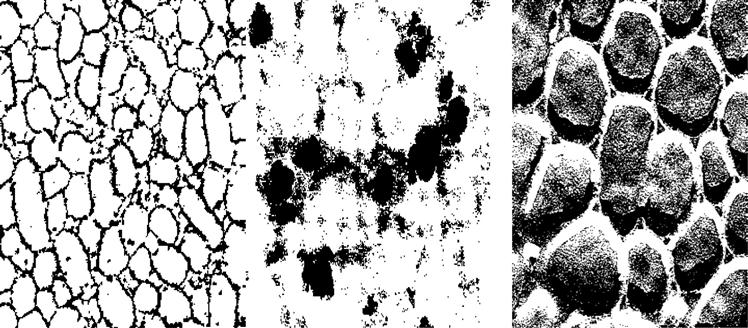
A chiton contains many one-dimensional magnetic wires in its teeth and tongue. They are composed of many magnetic columns, inside which is a collection of single-domain particles, and their biological function may not be limited to enhancing the wear resistance of its teeth and tongue. Interestingly, it has a natural template for nanowire growth. In the mineralized teeth of organisms, there is a network of organic fibers that serve as the nanowire growth template. Figure 5.1 shows the template cross-section and the formation process of magnetic material within.
At present, our understanding is insufficient regarding the synthesis of natural nanomagnetic particles in vivo; this is a topic that requires research efforts in the fields of biology, physics, and magnetics.
5.1.2 Classification of Magnetic Nanomaterials [3]
According to its applications, magnetic nanomaterials are divided into the following categories.
1. Nanocrystalline soft magnetic materials
Nanocrystalline soft magnetic materials are produced in large quantities and varieties and are applied in electricity, telecommunications, and home appliances. Representative of the products are Fe73.5CuNbSi13.5B8 (finement) with high saturated magnetization, as well as nanocrystalline Fe–M–B, Fe–M–C, Fe–M–N, Fe–M–O and other nanocrystalline soft magnetic series, where M can be Zr, Hf, Nb, Ta, V, and other elements. Their applications mainly include high-density magnetic heads, various types of transformers, magnetic switches, sensors, high-frequency micropower switches, and noise filter products.
2. Nanocrystalline permanent magnetic materials
Nanocrystalline permanent magnetic materials are represented by Nd2Fe14B,ThMn12, Sm2Fe17Nx, Sm2Fe17C, and Sm–Co–B (which has high thermal stability and good corrosion resistance). These materials are mainly used in electro-acoustic machines and mineral processing.
3. Nanomagnetic recording materials
Depending on their form, magnetic recording materials include granular and continuous thin film materials. They can be divided into two categories by nature as metallic and nonmetallic materials. Typical products include CrO2 and ferroalloy in the 1980s, Co-doped BaFe12O19 in the 1990s, and FeN, FeC, g-Fe2O3, CrO2, Co-g-Fe2O3, and Fe, BaFeOx, in the 2000s.
4. Ferro fluid
Ferro fluid is composed of magnetic particles (<10 nm) plus surfactant and base solution. The main products are magnetic particles that have already matured in the 1960s, namely Fe3O4 (10 nm) Co, Ni (<6 nm), and its alloys or nitrides. Common base liquids are water, kerosene, alkyl, ester, polyphenyl, silicone, and Dover carbon. The special feature of magnetic fluid is that magnetic particles in it can be magnetized in magnetic fields, and they are movable. It is mainly used in high-speed rotating shaft seals, lubricants, loudspeakers, damping devices, and density separation.
5. Granular perpendicular medium
Granular perpendicular medium is currently in the developmental stage and may be used in high-density magnetic recording and magnetic sensors. The recording layers of hard disks that are commercially used today are mainly made from CoCrPt–SiO2 materials. CoCrPt can be used as perpendicular recording media. When used as a perpendicular recording media, the recording layer is formed by epitaxial growth with Ru as the substrate, and the magnetic film formed is the granular film. It is now generally agreed that the role of exchange coupling between the internal film grains is a major source of noise, so nonmagnetic SiO2 is used to isolate the magnetic particles, so that no interaction force from coupling exchange will exist between magnetic particles and, hence, reduce the noise.
6. Nanomagnetic refrigeration working fluid
Compared with the usual compressed gas refrigeration, magnetic refrigerators have advantages such as high efficiency, low power consumption and noise, small size, and no pollution. This opens a new avenue for food-freezing and refrigeration equipment. Magnetic refrigeration tends to develop from a low temperature to a high temperature. In the present studies, typical magnetic refrigeration fluids include Gd, La–Ca–Mn–O, and Gd5Si2Ge2 materials.
7. Giant magnetoresistance
In a certain magnetic field, the resistance rapidly decreases at a ratio more than 10 times that of normal magnetic substances; this is a phenomenon is called GMR (see the following text). GMR materials have essential applications in magnetic sensor parts, high-density read heads, magnetic storage devices, numerical control machine tools, noncontact switches (magnetic switches: speed and position measurement for the automatic control anti-theft alarm system, car navigation, ignition devices), rotary encoders, MRAM (no power source to retain information), disks, and weak magnetic field detectors (10−2 to 10−6 T).
8. Nanoceramic material
Nanoceramic material mainly refers to nanometer-sized materials, such as Al2O3, ZrO2, SiC, and Si3N4. Their features are hardness, good wear resistance, excellent chemical stability (anti-oxidation, anti-fatigue), low density, and resistance to high temperatures. Nanoceramic materials are mainly used in microelectronics and quantum devices (computer boards). This application requires materials to have a small size, spherical shape, narrow size distribution, and nonagglomeration with high purity.
Synthesis of nanoceramic materials is mainly performed by means of gas-phase synthesis and sol gel synthesis, which allow the materials to have sintering densification and can be performed under high pressure at low temperatures, resulting in in situ self-reinforcement. NanoSiC is one of the typical representatives.
9. Raw materials for nanoprecision polishing
Raw materials for nanoprecision polishing can be used for some special window materials or multilayer interference film to improve optical performance, or can be used to improve electrical properties of piezoelectric materials, sensors, and so on. In addition, they can also be used in cell separation technology or used as a catalyst, as well as in specialty functional coatings (resistant to pollution, dust, wear, and fire).
10. Ceramic-based nanocomposites
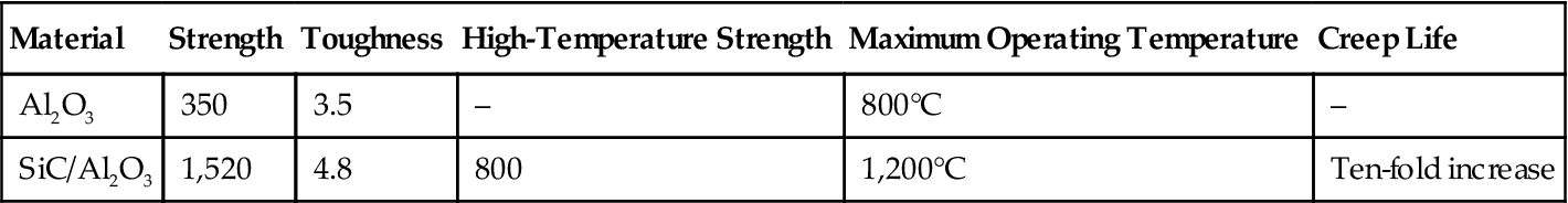
Nanoceramic particles dispersed in an inorganic matrix can enhance their performance. Table 5.1 shows the comparative data regarding the performance of Al2O3 before and after composition.
Table 5.1
Nanoceramic Particles Dispersed in Inorganic Matrix to Strengthen its Performance
| Material | Strength | Toughness | High-Temperature Strength | Maximum Operating Temperature | Creep Life |
| Al2O3 | 350 | 3.5 | – | 800°C | – |
| SiC/Al2O3 | 1,520 | 4.8 | 800 | 1,200°C | Ten-fold increase |
Nanoceramic particles dispersed in polymer matrix can be effective in modifying the performance. Table 5.2 shows a comparison between the data of the performance of Al before and after composition.
Table 5.2
Nanoceramic Particles Dispersed in Polymer Matrix Can Be Effective in Modifying Performance
| Material | Tensile Strength (MPa) | Bending Strength (MPa) |
| Al+1.0 wt% Si3N4 | 180 | 147 |
| Al+15 wt% Si3N4 | 176 | 94 |
| Al | 102 | 67.8 |
Nanoceramic particles are a candidate for carriers for the growth of nanowhiskers and carbon nanotubes. For example, Si–CN powder may be a base for growing Si–C whiskers and carbon nanotubes.
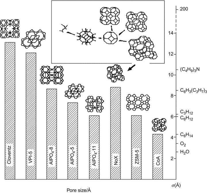
For ceramic-based nanocomposites, zeolite is a typical representative as the molecular sieve. Zeolite is an Si–Al-oxide that has a certain pore size and abilities in reversible absorption–desorption and distribution of the same size molecular sieve, ion-exchange capacity, and surface acidity. In 1756, Cronstedt (a Swedish chemist) discovered zeolite from minerals and gave it the current name. In 1930, McBain (a US scientist) found its selective adsorption characteristics, calling it molecular sieve. Artificial zeolite synthesis began in the 1950s (86 structures are already known). By 1992, the MCM series (Mobil) had been synthesized, in which MCM-41 has a hexagonal array of phase, MCM-48 is in the cubic phase, and MCM-50 is in the lamellar phase.
MCM-41 has the following characteristics: hierarchically organized structure, nanoadjustable porosity (1.5–30 nm, typically 4 nm), large pore aspect ratio, high surface area (up to 1,200 m2/g), as well as many changes in morphology and the composition of dense amorphous matrix (wall thickness of 1 nm), and higher thermal and water stability.
Figure 5.2 is a comparison of various zeolite pore sizes.
5.2 Basic Characteristics of Nanomagnetic Materials [1]
Among the three dimensions of a material, if any one dimension is within the range of 1–100 nm, then it is considered to be a nanomaterial. Nanomaterials are likely to exhibit one of the following common features: the quantum size effect, small size effect, surface effect, and macroscopic quantum tunneling effect (see Chapter 1).
In the magnetic domain structure and many other magnetic aspects, magnetic nanoparticles also show some other features.
5.2.1 Magnetic Domain
For bulk magnetic materials, the exchange interaction energy and magnetic anisotropy energy may cause parallel magnetic moments in their easy axis, but this will lead to a strong demagnetization energy.
For the radius R of a ball shape, demagnetization energy is
Ed=4π3μ0R3M2s6
(Ms![]() is the saturation magnetization).
is the saturation magnetization).
Obviously, the larger the size of R, the higher the demagnetization energy will be. To reduce energy, materials are bound to split into magnetic domains. But in the domain wall, as a transition zone between the two domains, magnetic moments are bound to deviate from the easy axis and adjacent magnetic moments are no longer parallel. The resulting domain walls can intervene in the total energy balance. For instance, a 180° domain wall may have an energy density given by
γ180=2√A1K1
(K1 is the anisotropy constant and A1 is the reduced exchange integral part, and the same is true for the next equation.)
In the nanoscale, nanoparticles will become single-domain particles. This is because when the particle size R is very small, the energy of domain walls can be stronger relative to the demagnetization energy. There is no need to make the sub-magnetic domains, and thus a single-domain particle forms. The critical size for the formation of single-domain particles can be estimated through the following methods [4]. The demagnetization energy of a single domain is set equal to the sum of domain wall energy and demagnetization energy by which two magnetic domains are divided, namely:
4π3μ0R3M2s6=4π3μ0R3M2s12+πR22√A1K1
assuming that after the single domain is split, the demagnetization energy is one-half of the single domain; the critical value of Rc ratio of the single domain is available as √A1K1/M2s![]() .
.
As far as nanothin films are concerned, if the magnetic film has a larger thickness, D, with magnetic moments rotating in the domain wall plane, the magnetic charge will not occur in the domain wall. The surface magnetic charge produces little effect of the demagnetization field. Such a phenomenon is called the Bloch domain wall. When there is a thin film, the surface magnetic charge with a demagnetization field cannot be ignored. Magnetic moments will be rotating in the film surface, that is, the film surface does not produce a magnetic charge; it is found in the domain walls and on both sides, known as the Neel domain wall.
For Fe–Ni film, D>100 nm indicates the presence of the Bloch domain wall; D<30 nm indicates the Neel domain wall, between which is the cross wall in a transitional state.
In theory, when D<12 nm, the film is a single domain. But a uniform demagnetization field in the film is difficult, so there is always a magnetic domain that will be generated.
5.2.2 Superparamagnetic Feature
With a volume of V, single-domain magnetic particles have anisotropy approximated as K1V (simplified as KV). When the magnetic particle size continues to decrease, the anisotropy barrier KV also will decrease accordingly. In this way, thermal motion energy kBT (simplified as kT) may exceed the anisotropy barrier KV and cause the orientation turnover of the magnetic moment, so that the magnetization direction of particles is presented as a magnetic performance in “Brownian motion,” with the total magnetization of particles aggregate as zero. This phenomenon is called superparamagnetism. It is characterized by coercivity:
Hc→0,asμHkBT≪1
Magnetization strength is given by
MP≈μ2H3kBT
where μ![]() is particle magnetic moment. A superparamagnetic feature is typically manifested by the magnetic ordering small-size effect of nanomaterials. Superparamagnetism can also be described by the Langevin function. The exception is that particles do not include a single atomic or molecular moment, but rather a collection of magnetic ordering. Magnetic orientation between the collections is arranged in confusion, showing the macroperformance of the “paramagnetism.”
is particle magnetic moment. A superparamagnetic feature is typically manifested by the magnetic ordering small-size effect of nanomaterials. Superparamagnetism can also be described by the Langevin function. The exception is that particles do not include a single atomic or molecular moment, but rather a collection of magnetic ordering. Magnetic orientation between the collections is arranged in confusion, showing the macroperformance of the “paramagnetism.”
For superparamagnetic colloidal particles in suspension, particles have only a weak effect of static magnetic and the Van der Waals force between them. As a result of the thermal motion, the magnetization vector within the particles can be rotated not only by overcoming the barrier of magnetic anisotropy energy but also by having motion as a whole. This is the magnetic fluid.
With a thermal motion energy kT, particle magnetic moment Ms with volume V can cross the barrier KV of anisotropy energy of K at a probability of p=exp(–KV/kT). That is, the original collection of consistent magnetic particles, after a period that is long enough, can be attenuated to the remnants of zero, with the relaxation time τ=(1/f0)exp(KV/kT), and frequency factor f0=109 s−1.
If you have to wait a year (107 s) before a decay process becomes “paramagnetic”, then this material cannot be superparamagnetic. So, τ is the relative standard. For instance, τ<10−1 s can be used for the superparamagnetic standard. Clearly, τ is relevant to the material anisotropy K, the temperature T, and the particle diameter D=V−3. In the case that the particle size V is fixed, only when particles attain a certain critical temperature T0 or higher can they be expressed as superparamagnetic; here, T0 is called the cut-off temperature. At a fixed temperature (e.g., room temperature), for the paramagnetic particles to show the performance of surplus they must have a size less than the critical size of V0.
The following are some superparamagnetic data in actual cases:
T=100 K, K=107 J/m3; if the material size is 6.3 nm, then the particle relaxation time τ=10−1 s; if size is 6.8 nm, then τ=101 s, and if particle size is 7.6 nm, then τ=10+5 s (or 1 day!). It is shown that the range for ultra-paramagnetic performance is rather narrow.
The following material sizes are required to show superparamagnetic features at room temperature: spherical iron, 12 nm; ellipsoid iron, 3 nm; HCP cobalt, 4 nm; and face-centered cubic cobalt, 14 nm.
Acquiring standardized data for different materials is essential, because different measurement methods may lead to different results. Under the condition that measurement time for data acquisition t<τ, the hot-fluctuation effect is not observed, and the material only shows the property of the usual single domain. Only when t>τ can superparamagnetism be clearly observed. For example, the time for Mossbauer measurement is 10−8 s, whereas part of the static magnetic measurements may have a time t=1–100 s.
5.2.3 Exchange Interaction
Exchange interaction is an equivalent interaction between particles in a microscopic identical multiparticle system. It reflects the indistinguishability of identical particles. Being a pure quantum effect, there is no corresponding classical concept for it. Nanomagnetic materials can be found within the normal magnetic exchange interaction; however, between the magnetic nanoparticles, nanomultilayer films, and one-dimensional magnetic wires, the availability of the exchange interaction and the relevant results are our concern.
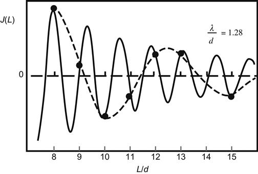
Here is an example to further expand on this theory. For magnetic multilayers, magnetic layers may have exchange coupling through a nonmagnetic metal layer, such as iron whiskers, which use a wedge-shaped gold laminate to complete the exchange coupling with another iron layer. Scanning electron microscopy with polarization analysis shows that the ferromagnetic exchange coupling is performed because of shock from changes in the ferromagnetic and antiferromagnetic layers in accordance with the thickness of the gold laminate. This shocking cycle has two cycles: short cycle and long cycle. A short cycle is approximately half of the Fermi wavelength, that is, λF/2, with the same expectations from the RKKY exchange model. Here, RKKY stands for the exchange interaction model of Ruderman–Kitter–Kasuya–Yosida. The basic characteristics include 4f electrons being localized, 6s electrons swimming, and f and s electrons in exchange interaction, so that the s electron is polarized. The spin of the polarized s electron may affect the orientation of the f electron spin. The result is the formation of a swimming s electron as medium, so that the 4f localized electron spin in magnetic atoms (or ions) produces exchange interaction with the 4f electron spin of its neighboring magnetic atoms. This is an indirect exchange interaction. The RKKY model is applicable for rare earth. The reason for the formation of the long-period shocks may lie in the experimental methods, which were observed in a discontinuous nature, taking a single atomic layer as a single observation unit, rather than the continuous change of the thickness; the results are from intermittent sampling, as shown in Figure 5.3.
This research on exchange coupling led to the discovery of the GMR effect and its further development as the base for spintronics research. Between antiferromagnetic and ferromagnetic layers, exchange coupling can be firmly attached to the ferromagnetic layer. This method has been widely used in GMR device designs.
Nanocrystalline exchange may lead to random anisotropy. Because the magnetic nanograin size D is less than the exchange length Lex, the exchange coupling between grains will effectively offset the local random anisotropy K, and the average density of anisotropy energy <K> tends to be zero as the scale D gets smaller. As <K>=K1/N1/2, the number of grains contained in the context of the exchange length N=(Lex/D)3. So, <K>=K1(D/Lex)3/2, and the ferromagnetic exchange length is subject to the relation Lex=(A/![]() K
K![]() )1/2. Therefore, the random anisotropy, <K>=K14D6/A3, that is, <K>, declines in the six orders of magnitude as D decreases, and the corresponding magnetic permeability, μ, also increases by six orders of magnitude as the nanoscale of particles decreases.
)1/2. Therefore, the random anisotropy, <K>=K14D6/A3, that is, <K>, declines in the six orders of magnitude as D decreases, and the corresponding magnetic permeability, μ, also increases by six orders of magnitude as the nanoscale of particles decreases.
The flexible exchange coupling between soft particles and hard magnetic particles can be used to maintain a high Hc![]() and Br, thereby enhancing the hard magnetic properties.
and Br, thereby enhancing the hard magnetic properties.
5.2.4 Coercivity Hc
Already introduced in the previous sections, the understanding of coercivity tends to be very complex with the changes in particle size. When the particles become as small as single-domain scale, the antimagnetization process is in either a homogeneous or inhomogeneous rotation process of the magnetic moment. Hc![]() is proportional to (K/Ms) of the materials (K for the anisotropy constant). This is one of the ways to get a higher Hc
is proportional to (K/Ms) of the materials (K for the anisotropy constant). This is one of the ways to get a higher Hc![]() , namely the hard magnetic properties of the material. However, nanomagnetic materials may have a smaller Hc
, namely the hard magnetic properties of the material. However, nanomagnetic materials may have a smaller Hc![]() simply by means of anisotropic exchange interaction that makes a very small average anisotropy <K> with a scale less than the exchange length. As the particle size is reduced to the superparamagnetic critical size, the coercivity approaches zero.
simply by means of anisotropic exchange interaction that makes a very small average anisotropy <K> with a scale less than the exchange length. As the particle size is reduced to the superparamagnetic critical size, the coercivity approaches zero.
Figure 5.4 shows several specific materials and the relationship between the coercivity and particle size.
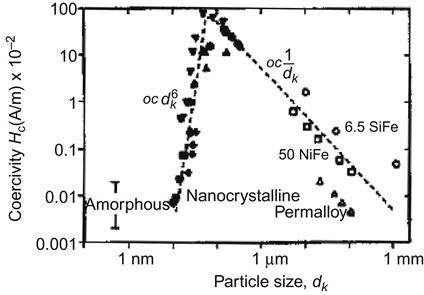
 and particle size dk
 . From Ref. [1].
5.2.5 Curie Temperature
Curie temperature Tc![]() is an important parameter of magnetic materials, usually directly proportional to the exchange integral A, but also related to the material configuration and spacing of the atoms. In nanomaterials research, the Curie temperature is found to decline with the decrease of nanoscale particles or thin films because of the small size effect and the surface effect. The lack of interaction between surface atoms and the small scale may also lead to smaller atomic spacing. All this may cause a decline of the exchange integral A, resulting in a decline of Curie temperature. For example, for 5 nm Ni, lattice parameters shrink by 2.4%.
is an important parameter of magnetic materials, usually directly proportional to the exchange integral A, but also related to the material configuration and spacing of the atoms. In nanomaterials research, the Curie temperature is found to decline with the decrease of nanoscale particles or thin films because of the small size effect and the surface effect. The lack of interaction between surface atoms and the small scale may also lead to smaller atomic spacing. All this may cause a decline of the exchange integral A, resulting in a decline of Curie temperature. For example, for 5 nm Ni, lattice parameters shrink by 2.4%.
5.2.6 Susceptibility
Magnetic properties of nanoparticles are closely related with the parity of the total number of electrons contained. Electrons with an odd number follow the Curie–Weiss susceptibility law:
χ=CT−Tc (5.1)
Because of the quantum size effects, susceptibility complies with the law of d−3 (d for an average particle diameter), whereas the magnetic susceptibility of electrons with an even number is subject to:
χ∝kBT (5.2)
Susceptibility complies with the d2 law (see Chapter 1).
Obviously, the basic common characteristics of nanomaterials and several special aspects of magnetic materials are different from those of bulk materials. By harnessing these features, we can create many novel materials with special properties beyond that of the bulk materials.
5.3 Some Specific Nanomagnetic Materials
This section describes a number of specific nanomagnetic materials, including zero-dimensional magnetic fluids and magnetic microspheres, one-dimensional magnetic nanowires and their arrays, two-dimensional magnetic nanothin film and its applications, nanocrystalline soft magnetic materials and their industrialization, double-phase nanocomposite hard magnetic principles, and the idea of high-frequency and microwave nanomaterials.
5.3.1 Magnetic Fluids [5]
Magnetic fluids are a stable colloidal system formed by the nanoscale (10 nm or less) strong magnetic particles highly dispersed in a liquid. In the 1960s, the United States first used them in the aerospace industry, which then found their way into commercial applications. Now, a huge industry has been developed. Magnetic fluid businesses can be found in the United States, Japan, Germany, and other developed countries, with the world’s annual production being millions of tons of magnetic fluid devices.
Magnetic fluid is composed of strong magnetic particles, base liquid, and surface-active agent. In it, the magnetic particles must be very small to render the chaotic Brownian motion in the base fluid. Such a thermal motion may offset the gravity sedimentation and produce a loss of electricity and magnetism in the role of the mutual cohesion between particles. Meanwhile, under the actions of gravity, electricity, and magnetic fields, it can be viable without producing precipitation and condensation. As with iron, the particle diameter should be less than 3 nm; for Fe3O4, the diameter is not allowed to exceed 10 nm. Magnetic particles and the base fluid are mixed into one, presenting combined features that are shared by general magnetic materials and the liquid with mobility. It boasts several unique properties.
There are different ways for the preparation of nanoparticles, of which chemical coprecipitation technology features the following advantages: easy operation, low cost, less demanding on the equipment, and so on. Selection of suitable surface-active agents is the key to preparation of magnetic fluids. Surfactant-coated surfaces of the particles can bring about the following effects: preventing the oxidation of magnetic particles; overcoming the cohesion of the particles caused by van der Waals forces; weakening the static magnetic attraction; and changing the nature of the surface of magnetic particles, so that particles and the base can be mixed into a single fluid. The general requirement for the surface-active agent is that one side of the active agent can be adsorbed onto the surface of particles, forming strong chemical bonds, whereas the other side can become soluble with the base liquid. Each of the base fluids requires different surface-active agents, and sometimes they even require two or more surfactants. Table 5.3 shows a variety of magnetic fluid properties and compositions.
Table 5.3
Composition and Properties of Magnetic Fluid
| Magnetic Particles | Surfactant | Containing Liquid | Density (gcm−3) | Degree of Particles within a Unit of /cm−3 Volume | Saturation Magnetization Mg/T(G) | Chemical Stability of the Atmospheric Environment |
| Fe3O4 | Oleic acid | Synthetic oil | 1.23 | 0.0438 (438) | Better | |
| Mn0.2Fe2.8O4 | Oleic acid | Kerosene | 1.31 | 0.052 (520) | Better | |
| Co | Polybutadiene amber imide | Toluene | 2.77×10¹⁷ | 0.0384 (384) | Poor | |
| 11.3×10¹⁷ | 0.107 (1,070) | |||||
| Fe | Polybutadiene amber imide | Lubricants | 1.07 | 0.0448 (448) | Poor | |
| 1.24 | 0.0767 (767) | |||||
| ε-Fe3N | Polyamines | Kerosene | 1.19 | 8.8×10¹⁶ | 0.117 (1,170) | Better |
| 2.04 | 3.4×10¹⁷ | 0.233 (2,330) | Better |

Magnetic fluids are magnetic and have mobility, and have unique magnetism, fluid mechanics, and optical and acoustic properties. Magnetic fluid is presented with superparamagnetic zero intrinsic coercivity, and there is no residual magnetism. Magnetic fluid magnetized in an outer magnetic field satisfies the modified Bernoulli equation. Compared with the conventional Bernoulli equation, magnetic energy is added so that magnetic fluid accompanies novel magnetic-associated properties that make it unique. For example, the apparent density of magnetic fluid increases as the external magnetic field strength increases; as light passes through the diluted magnetic fluid, it will produce the light birefringence effect and a two-way color phenomenon. When the magnetic fluid is magnetized, the optical anisotropy will occur relative to the magnetic fields. Polarized light with the electric vector parallel to the direction of the external magnetic field is absorbed more perpendicular to the direction, with a higher refractive index. When ultrasound is transmitted in magnetic fluid, its speed and attenuation are associated with the external magnetic field, showing anisotropy; magnetic liquids in an alternating field have a frequency dispersion of magnetic permeability, magnetic viscosity, and so on.
The special nature of magnetic fluid has opened up many new fields of application. Some of the technical difficulties in the past have been resolved because of its emergence. The following is a brief introduction to the application of several of its principles.
1. Dynamic sealing technology
The dynamic sealing technology in the rotation axis is one of the comparatively mature and the most important applications of magnetic fluid, now widely used in shaft seals for precision instruments, such as X-ray rotating anode diffractometer, crystal furnace, high-power lasers, computers, and so on. In the nonuniform magnetic field, magnetic fluid will be gathered in the largest magnetic field gradient. Therefore, the outer magnetic field can be used to constrain the magnetic fluid in a sealed part, forming an “O” ring of magnetic liquid, showing properties of no leakage, no wear and tear, self-lubrication, and long life.
Currently, precision instruments all include a magnetic fluid sealing component. Such an instrument generally costs $2,000 to $3,000, and the magnetic fluids used in them are not sold separately. Magnetic fluid sealing technology is important for sealing of vacuums and gas dynamic instruments and sealing out dust. However, it is seldom used in sealing water because of some practical difficulties. If breakthroughs could be made regarding the closure of water and oil sealing, then its applications would be extremely broad and bring about huge economic and social benefits.
2. Audio speakers
Injecting magnetic fluid into a speaker’s voice coil gap may have a certain damping effect on the movement of voice coil and enable it to automatically locate. At the same time, the heat generated by it can be dissipated through the magnetic fluid. Therefore, adding magnetic fluid can help improve the speaker’s power load. With the same structure design, the input power can be increased twofold, while the frequency response and fidelity can be enhanced. Using magnetic fluids in metal brane speakers can enhance the performance more significantly. At present, the production lines and magnetic fluids that many manufacturers of magnetic fluid speakers in China use are imported from abroad. If we can produce magnetic fluid ourselves, then the cost of such products can be substantially reduced.
3. Damping devices
Magnetic fluid can be used as a rotary and linear damper to damp the additional oscillation modes of the system. Compared with general damping media, magnetic fluids can be localized with the help of the external magnetic field. For example, in a stepper motor, magnetic fluid damping can be used to eliminate the vibration and resonance in the system to ensure precise positioning of the motor. In addition, the use of magnetic fluid damping in the vibration isolation tables is able to eliminate noise interference from the external vibration to ensure the proper work of precision instruments (scales, optical equipment, and so on).
4. Mineral separation
The apparent proportion of magnetic fluid may change with the changes of an external magnetic field. This characteristic can be used to filter nonmagnetic minerals in different proportions. Minerals with the proportion difference of 10% can be well separated using this technique. In this process, water-based magnetic fluids are normally used, and they can be reused.
5. Switching function
Mercury and magnetic fluid can be placed in a nonconductive container, where the magnetic field is applied to change the location of mercury to achieve the purpose of switching on and off the electric current. Magnetic fluid can be sealed in a nonmagnetic container on the shaft. While the rotor is stationary, the magnetic fluid stays in the lower part of the container, so the sensor cannot detect it; when the shaft rotates, centrifugal force distributes the magnetic fluid on the container wall. Then, the sensor detects the magnetic fluid and causes a switching action.
6. Precision grinding and polishing
Magnetic fluid grinding harnesses magnetic fluid’s buoyancy: micron abrasions are suspended on a liquid surface, allowing close contact with the work piece to be polished. No matter how special the surface shape of a work piece is, this technology is applicable for precision polishing. It may also be used to grind high-quality Si3N4 ceramic balls with efficiency 40 times higher than that of traditional methods.
7. Magnetic fluid sensors
There are two kinds of commercially available magnetic fluid sensors: one is used in the oil exploration industry to measure acceleration and tilting of drill bits, and the other is used in the construction industry to detect the tilting of underground pipes.
8. Other applications
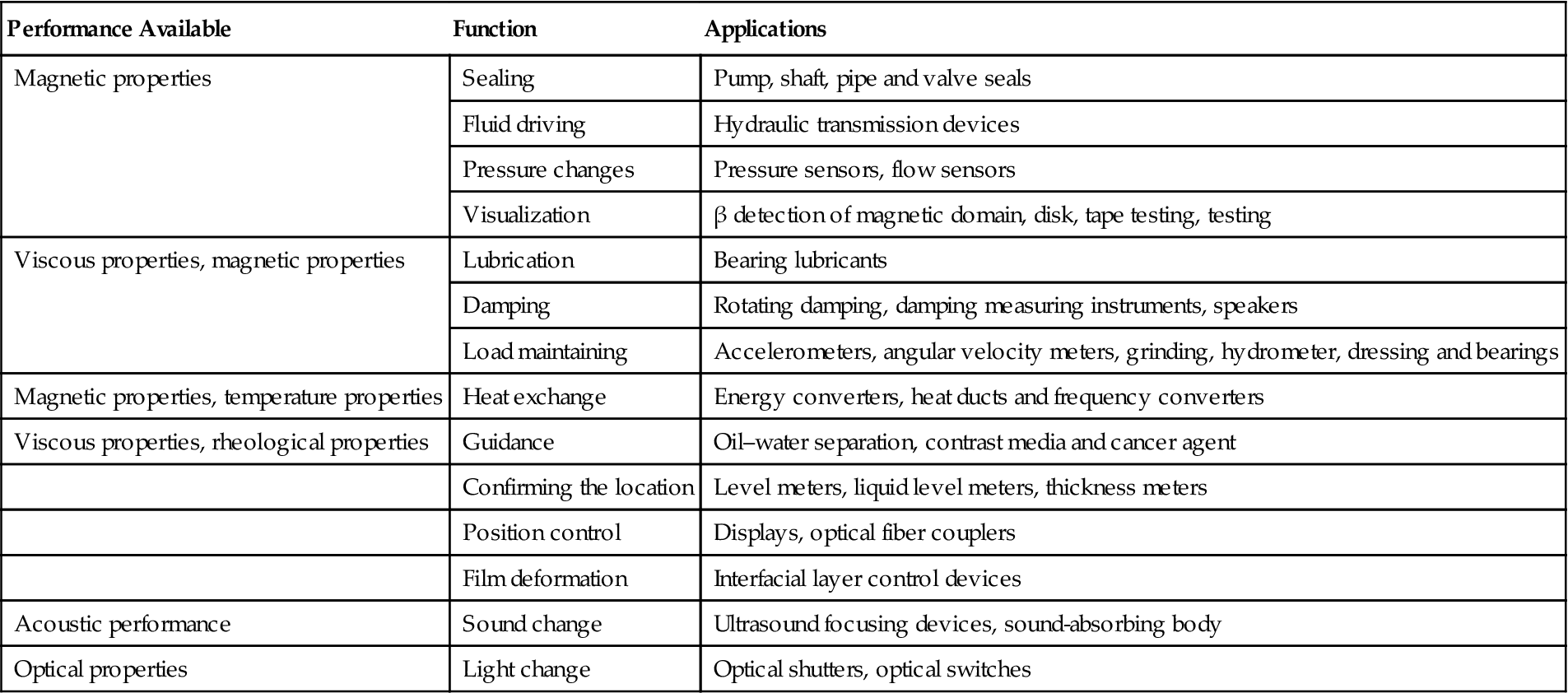
In addition, magnetic fluid has a bright future in many areas, such as magnetic fluid printing, magnetic fluid film bearings, sonar systems, magnetic substances, magnetic cell separation, artificial heaters with magnetic fluid, turbine power generation with magnetic fluid, optical switches, magnetic fluid brakes, and so on. Properties and applications of magnetic fluids are shown in Table 5.4.
Table 5.4
Properties and Applications of Magnetic Fluid
| Performance Available | Function | Applications |
| Magnetic properties | Sealing | Pump, shaft, pipe and valve seals |
| Fluid driving | Hydraulic transmission devices | |
| Pressure changes | Pressure sensors, flow sensors | |
| Visualization | β detection of magnetic domain, disk, tape testing, testing | |
| Viscous properties, magnetic properties | Lubrication | Bearing lubricants |
| Damping | Rotating damping, damping measuring instruments, speakers | |
| Load maintaining | Accelerometers, angular velocity meters, grinding, hydrometer, dressing and bearings | |
| Magnetic properties, temperature properties | Heat exchange | Energy converters, heat ducts and frequency converters |
| Viscous properties, rheological properties | Guidance | Oil–water separation, contrast media and cancer agent |
| Confirming the location | Level meters, liquid level meters, thickness meters | |
| Position control | Displays, optical fiber couplers | |
| Film deformation | Interfacial layer control devices | |
| Acoustic performance | Sound change | Ultrasound focusing devices, sound-absorbing body |
| Optical properties | Light change | Optical shutters, optical switches |
5.3.2 Magnetic Microspheres
With the help of the surfactant, nanomagnetic particles can be combined with monoclonal antibodies, enzymes, drugs, and genes known as magnetic microspheres, which have exhibited important application prospects in bioengineering, biochips, biomolecular labels, and so on. In addition, they can create targeting mechanisms in drugs, turning them into so-called biological missiles. Such drugs are effective in the treatment of cancers.
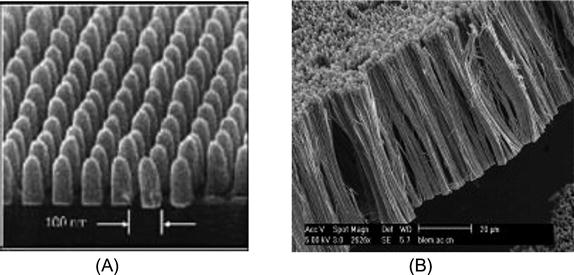
5.3.3 One-Dimensional Nanowires
The overall trend of the development of computer disks is decreasing in size while increasing rapidly in storage density. Common disks have a storage density of 106 to 107 bits/in.2. With the advent of CD-ROM, the storage density increased to 109 bits/in.2. Because of limitations of the properties of materials, 1011 bits/in.2 was once considered to be the limit of disk storage density.
Research and development of a new generation of ultrahigh-density magnetic recording materials have attracted the attention of many researchers. One-dimensional magnetic nanowires have developed rapidly in recent years and are a hot research topic. These materials can be made of a single metal, alloy, compound, complex, or multilayer film. Figure 5.5 shows typical examples of one-dimensional magnetic nanowires. Nanoquantum storage medium prepared with these provides a direction in the development of high-density and low-noise hard disk medium. In recent years, quantum dot-matrix thin film has become popular in this area. Specifically, magnetic metal or alloy is injected into the nonmagnetic media to obtain a quantum dot-matrix thin film isolated from each other. The basic idea of this approach is as follows. A template is first made to have a high pore density and controllable aspect ratio; then, magnetic metal or composite magnetic materials are injected into its microholes to form ordered nanowire arrays. As nanomagnetic units on the film are separated from each other, the film structure in this array is also known as a quantum magnetic disk (QMD). In comparison with conventional disks, QMDs possess the following advantages: the spontaneously quantified magnetic moment of each bit; precise location is not required on the write head in the quantization process; small, isolated, smooth transfer area that ensures high recording density and transmission noise approximating 0; and precise positioning of the read–write head to overcome the superparamagnetic limit. Chou et al. [6] injected magnetic material of 50 nm or less into the ordered nonmagnetic porous medium and obtained the QMD structured nanowire arrays with corresponding recording density up to 400 Gbit/in.2 or higher. In 1997, the first nanostructured disk was successfully developed by means of nanolithography in the Laboratory of NanoStructures in the Department of Electronic Engineering, University of Minnesota. This kind of disk has a size of 100×100 nm2, which is the quantum wire array of cobalt rod based on a cycle of 40 nm by diameter of 100 nm and length of 40 nm. It has a storage density of 4×10¹¹![]() bits/in.2. After that, other scientists, such as those at MIT, also claimed that they made quantum disks of nanostructures [7].
bits/in.2. After that, other scientists, such as those at MIT, also claimed that they made quantum disks of nanostructures [7].
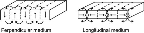
Traditionally, magnetic data storage uses the technique of horizontal recording. As its name implies, the data bits are arranged horizontally (parallel to the disk surface). The use and evolution of this recording mode have lasted 50 years. However, the increased rate of storage density of this method slowed since the beginning of the twenty-first century because it has physical limits, for example the superparamagnetic effect. This has resulted in the recording density decreasing to an annual growth of 50–60% or even slower. In contrast with this mode, the data bits in perpendicular magnetic recording are aligned vertically (data bits perpendicular to the disk). Perpendicular recording mode (PRM) (Figure 5.6) can easily overcome the superparamagnetic effect, making it possible to achieve larger disk space for more data and, hence, to reach a higher areal density. In recent years, perpendicular magnetic recording mode has attracted widespread concern. Nanowire array is an important candidate for perpendicular magnetic recording material.
Quantum wire arrays can also be used for cell separation, and have shown purity of 80% and yield up to 85%.
5.3.4 Two-Dimensional Films [1]
Research on two-dimensional magnetic nanothin film has attracted much attention in recent decades. In the 1960s, there was a boom of studies on NiFe film, which was mainly used in magnetic memory and later replaced by semiconductors; in the 1970s, the research was focused on the magnetic bubble film, which had trial applications in magnetic storage and was later eliminated for various reasons. The 1980s witnessed the climax of a research campaign for magneto-optical film, which serves as the basis for the rewritable CD-ROM in the current market. By the 1990s, research on magnetic multilayers led to the discovery of the GMR effect and the emergence of a new discipline, spintronics.
In magnetic multilayers, the GMR effect works via a mechanism that spin-polarizes electrons; within the scope of its coherence length, it may have different scattering probabilities in different spin orientations of the film, that is, different resistances. The GMR spin-valve structure is one practical design. The spin-valve structure with nano-oxide layers is a finalized product (readout heads).
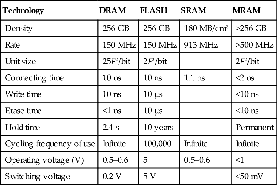
After the GMR discovery, tunneling magnetoresistance (TMR) was discovered in 1995, with magnetoresistive random access memory (MRAM) as one of its important application prospects. MRAM is a nonvolatile computer memory (NVRAM) technology that began its development in the 1990s, and amazing progress has been made ever since. Supporters of the MRAM technology believe that MRAM will eventually become dominant and supersede all other types of memory, becoming a true “universal memory” (Table 5.5).
Table 5.5
MRAM Compared with the Current Memories (F is Feature Size)
| Technology | DRAM | FLASH | SRAM | MRAM |
| Density | 256 GB | 256 GB | 180 MB/cm2 | >256 GB |
| Rate | 150 MHz | 150 MHz | 913 MHz | >500 MHz |
| Unit size | 25F2/bit | 2F2/bit | 2F2/bit | |
| Connecting time | 10 ns | 10 ns | 1.1 ns | <2 ns |
| Write time | 10 ns | 10 μs | <10 ns | |
| Erase time | <1 ns | 10 μs | <10 ns | |
| Hold time | 2.4 s | 10 years | Permanent | |
| Cycling frequency of use | Infinite | 100,000 | Infinite | Infinite |
| Operating voltage (V) | 0.5–0.6 | 5 | 0.5–0.6 | <1 |
| Switching voltage | 0.2 V | 5 V | <50 mV |
5.3.5 Magnetic Nanocomposite Materials [1]
Magnetic nanocomposite material is one research target with very practical values. Because of the flexibility and availability of materials and performance tuning, suitable material recipes can be found in various areas. Stealthy materials in nanoresearch also take priority and include nanomagnetic composite particle films and nanomagnetic multilayers. A few examples of other magnetic materials are also described in this chapter.
After annealing the amorphous FeSiB, Cu and Nb are doped to control the grain size, and the resulting novel nanocrystalline soft magnetic materials may have a changing law that is totally different from that in conventional soft magnetic materials—small coercivity plus high magnetic permeability rate.
The mechanism in nanocrystalline soft magnetic material is represented in the exchange coupling interaction between nanograins, which can effectively offset the partial and random anisotropy. The average anisotropy energy density <K>=K1/N, and the length scope of this exchange contains the number of grains N=(Lex/D)3. So, <K>=K1(D/Lex)3/2, and the ferromagnetic exchange length is subject to the relation Lex=(A/![]() K
K![]() )1/2. Because the grain size D is less than Lex, its random anisotropy can be expressed as <K>=K14D6/A3, for example <K> and D are subject to six orders of magnitude. Accordingly, magnetic permeability μ, with the decrease of the nanoparticles in the size D, also increased six orders of magnitude (Table 5.6).
)1/2. Because the grain size D is less than Lex, its random anisotropy can be expressed as <K>=K14D6/A3, for example <K> and D are subject to six orders of magnitude. Accordingly, magnetic permeability μ, with the decrease of the nanoparticles in the size D, also increased six orders of magnitude (Table 5.6).
Table 5.6
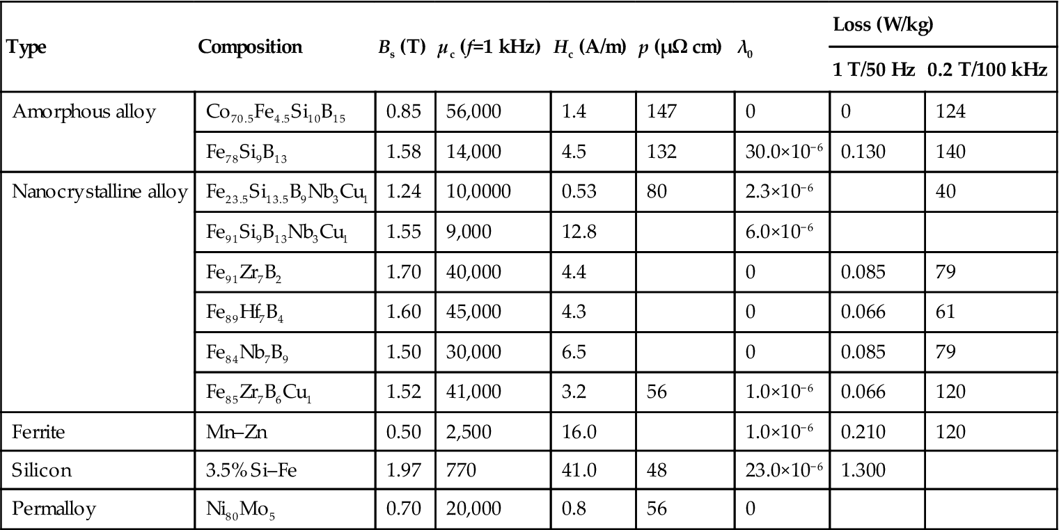
Comparison of the Novel Soft Magnetic Alloy with Traditional Materials on Magnetic Properties
| Type | Composition | Bs (T) | μc (f=1 kHz) | Hc (A/m) | p (μΩ cm) | λ0 | Loss (W/kg) | |
| 1 T/50 Hz | 0.2 T/100 kHz | |||||||
| Amorphous alloy | Co70.5Fe4.5Si10B15 | 0.85 | 56,000 | 1.4 | 147 | 0 | 0 | 124 |
| Fe78Si9B13 | 1.58 | 14,000 | 4.5 | 132 | 30.0×10⁻⁶ | 0.130 | 140 | |
| Nanocrystalline alloy | Fe23.5Si13.5B9Nb3Cu1 | 1.24 | 10,0000 | 0.53 | 80 | 2.3×10⁻⁶ | 40 | |
| Fe91Si9B13Nb3Cu1 | 1.55 | 9,000 | 12.8 | 6.0×10⁻⁶ | ||||
| Fe91Zr7B2 | 1.70 | 40,000 | 4.4 | 0 | 0.085 | 79 | ||
| Fe89Hf7B4 | 1.60 | 45,000 | 4.3 | 0 | 0.066 | 61 | ||
| Fe84Nb7B9 | 1.50 | 30,000 | 6.5 | 0 | 0.085 | 79 | ||
| Fe85Zr7B6Cu1 | 1.52 | 41,000 | 3.2 | 56 | 1.0×10⁻⁶ | 0.066 | 120 | |
| Ferrite | Mn–Zn | 0.50 | 2,500 | 16.0 | 1.0×10⁻⁶ | 0.210 | 120 | |
| Silicon | 3.5% Si–Fe | 1.97 | 770 | 41.0 | 48 | 23.0×10⁻⁶ | 1.300 | |
| Permalloy | Ni80Mo5 | 0.70 | 20,000 | 0.8 | 56 | 0 | ||
5.3.6 Double-Phase Nanocomposite Hard Magnets
Theory shows that the soft and hard nanocomposite magnetic particles will be integrated with the strengths of both higher soft magnetic Ms and hard magnetic Hc, thus forming a novel hard magnetic material with a nanomagnetic energy level twice as high as the best available NdFeB. That is, its magnetic energy level is expected to be almost twice as high as the current value. Its mechanism is based on the production of flexible exchange-coupled magnetic particles in the hard and soft particle interface.
For example, with diameter of D, soft magnetic balls surrounded by a hard magnetic medium are made as a model to SmCo/Fe. The relationship between the reversal magnetization nucleation field and the particle diameter is calculated. The result indicates that if particles are less than 3 nm in diameter, the nucleation field can be up to 19.5 T.
5.3.7 High-Frequency Microwave Nanomagnetic Materials
The particles or thin film in nanoscale, which is less than the thickness of the skin of electricity, is very conducive to high-frequency applications. Requiring more permeability with a higher real part μ′, the higher imaginary part μ″ may help to serve as stealth absorbing materials. If μ″ is so low that consumption is small, then it can be made to have similarly high-frequency soft magnetic and inductance materials.
Studies have shown that there is a Snoek limit in bulk materials regarding the frequency and magnetic permeability [8]. We provide simple proof of this here. We assume that its resonance mechanism is the natural resonance determined by the material anisotropy magnetic field ω=γHk![]() .
.
From Hk=2K1/Is![]() , we get
, we get
ω=2λK1Is(K1>0) (5.3a)
From Hk=−4K1/3Is![]() , we get
, we get
ω=−4λK13Is(K1<0) (5.3b)
Meanwhile, the magnetic permeability caused by the magnetization rotation, with a random distribution of the easy axis, can be expressed as
ˉμα=Is23K1μ0(K1>0) (5.4a)
ˉμα=−Is22K1μ0(K1<0) (5.4b)
Equation (5.3) is multiplied by Eq. (5.4), and we get
ωˉμα=2γIs3μ0 (5.5)
Obviously, for an identified material ωˉμα∝Is![]() is a constant.
is a constant.
With the presence of cubic anisotropy, no ferrite can have permeability higher than the limits of Snoek (Table 5.7).
Table 5.7
Restrictions of the Operating Frequency on the Magnetic Permeability
| f (MHz) | 1,120 | 560 | 280 | 140 |
| μ | 5 | 10 | 20 | 40 |
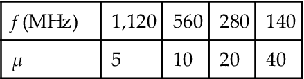
This absolute limit can be overcome with the support of planar anisotropy of nanothin film.
The easy plane in planar anisotropy is set to be vertical to axis c and magnetization anisotropy field in planar rotation is Hα1![]() ; the field is the anisotropy for magnetization to transfer out of the plane Hα2
; the field is the anisotropy for magnetization to transfer out of the plane Hα2![]() . Then, bulk materials in this planar anisotropy may have natural resonance frequency as follows:
. Then, bulk materials in this planar anisotropy may have natural resonance frequency as follows:
ω=γ√Hα1Hα2 (5.6)
For polycrystalline materials with an in-plane random distribution of the easy axis, rotational magnetic susceptibility is
ˉμα=Is23K1μ0=2Is3μ0Hα1 (5.7)
Equation (5.6) is multiplied by Eq. (5.7), and we get
ωˉμα=2γIs3μ0√Hα2Kα1 (5.8)
Experiments confirmed that the plane ferrite had an occurrence of natural resonance frequency that is higher than the Snoek limit. Therefore, the use of nanometer thin film materials enables the Snoek limit ωˉμα![]() to be increased by the fold of √Hα2/Kα1
to be increased by the fold of √Hα2/Kα1![]() . For the FeNi alloy film,
. For the FeNi alloy film,
Is=1.16T,K1=−2×10²Jm−3
And the line ratio
η=2000,√Hα2Kα1=63.345
If the film thickness is 10 nm, then the diameter of a circular thin film should be 20 μm. The use of material with high saturation magnetization can have ωˉμα![]() further enhanced.
further enhanced.
Because both the particle size and spacing are less than the length of exchange coupling, the exchange interaction between particles will average out the anisotropy of particles. Particle magnetization will be coupled together so that the whole film Hc is greatly reduced, and μ is greatly increased.
For instance, the nanogranular film (FeCo)-Zr2O5, at 1 GHz, μ′~260, μ″~320, is improved by two orders of magnitude compared with the conventional expected value (Figure 5.7).
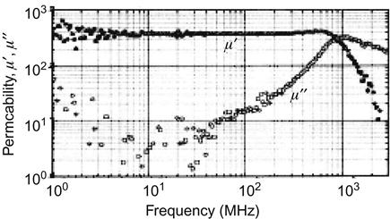
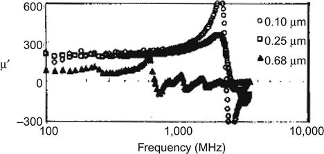
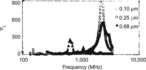
Nanoparticles or thin films with high-frequency characteristics can be used to produce high-frequency thin film inductors. It is important to address the miniaturization and integration of inductors that nanoparticles or thin film have higher high-frequency magnetic permeability μ′ and lower μ″ to produce a small loss. The specific requirements of the material are as follows: high electrical resistivity ρ; high magnetic permeability and low loss at 2,000 MHz or more; and good temperature stability up to 200°C. This requires the material resonance frequency fr to be higher than 2 GHz: fr=γ/2π(4πMsHk)1/2, where γ is the gyromagnetic ratio. Therefore, we must choose the right Ms, Hk and ρ. The following example illustrates the curve of the material CoZrNb on the real and imaginary parts of permeability versus frequency (Figures 5.8 and 5.9).
5.4 Preparation of Nanomagnetic Materials
5.4.1 Classification
Nanomagnetic materials can be expressed on a number of levels, for example zero-dimensional magnetic nanoparticles, one-dimensional magnetic nanowires, two-dimensional magnetic nanofilms, and the bulk of the magnetic nanoparticles complex. Preparation of nanomaterials can be divided into two categories: (1) top-down, that is, from big to small, whereby bulk materials are broken into nanoparticles or large areas are etched into the nanopatterns; and (2) bottom-up, namely small to large, whereby atoms and molecules are developed per the growth requirements into nanoparticles, nanowires, nanocomposite films, or nanoparticles (Figure 5.10).
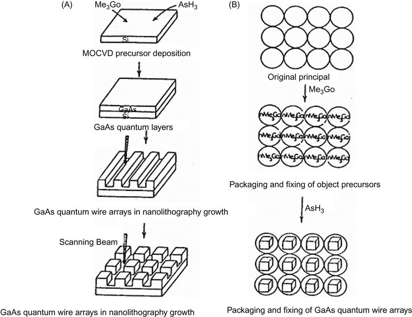
Table 5.8 shows another classification. More changes can be created for practical use.
Table 5.8
Classified Methods for Synthesis and Preparation of Some Commonly Used Nanomaterials
| Method | Examples |
| Gas phase | Gas condensation, active hydrogen–molten metal reaction, sputtering, ohmic heating evaporation, hybrid plasma, laser-induced chemical vapor deposition |
| Liquid phase | Coprecipitation, spray, hydrothermal mode, microemulsion, sol–gel mode, electro-deposition, solvent evaporation decomposition, high-pressure quenching |
| Solid phase | High-energy ball milling, noncrystallization, combustion synthesis |
5.4.2 Specific Instances [1]
Examples for the specific preparation of nanomaterials are described here.
5.4.2.1 Mechanical Crushing Method
Mechanical means, such as high-energy ball milling, ultrasonic or jet milling, and others, can have powder prepared into nanoparticles. This is an example of a top-down approach, which is suitable for refractory metals or materials beyond the use of chemical reactions. The disadvantages include the difficulties in classification according to the particle size and serious surface contamination.
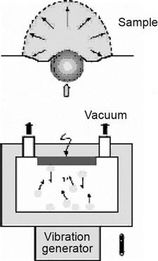
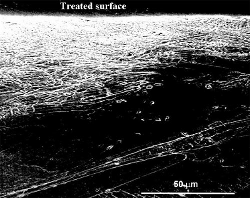
Bombarding a metal surface with high-energy balls makes it possible to turn the surface structure into nanoscale; this can improve the abrasion and corrosion resistance of the processed material. Meanwhile, the surface is identical to the bulk material, and thus it does not peel off like nanocoating material. The main mechanism of this method is to produce a large number of defects and dislocations, which further develop into dislocation walls, and thus cut the large crystals into nanocrystalline grains (Figure 5.11).
We can see from Figure 5.12 that dislocation density gradually decreases from the surface to the interior. It is the dislocation wall that cuts the large crystals into nanocrystalline grains.
5.4.2.2 Etching Method
Etching also follows the top-down approach, by which large areas of film, through chemical, electron beam, ion beam etching, or even atoms moving with the help of scanning tunneling microscopes and other equipment, are prepared into nanodots, nanolines, or other nanopatterns.
Etching treatment is commonly executed using lithography or an ion beam etching machine. SPM devices can be used for the atomic handling work, such as scanning tunneling electron microscopy and atomic force microscopy (see Chapter 2).
Corresponding to the top-down approach to manufacturing, nanomaterials are also able to begin growth from bottom to top, for example from atoms and molecules.
5.4.2.3 Physical Method
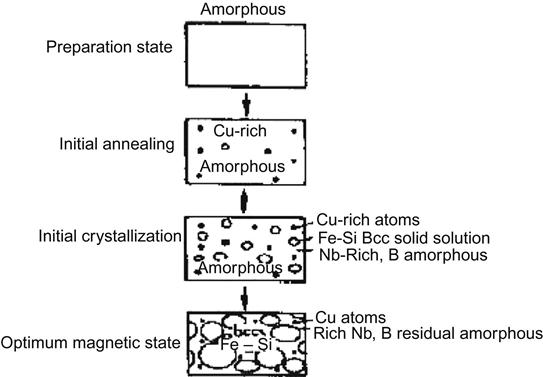
By using physical methods, there will be no chemical reactions in the preparation process. Commonly used methods are atomization, sputtering, evaporation, and noncrystallization. Gas coagulation is completed as follows: in a vacuum chamber filled with inert gas, the metal is heated, evaporating into the mist of atoms to collide with inert gas. This makes the metal lose momentum, and it is precipitated onto the liquid nitrogen-cooled rods. Then, this powder can be scraped off and collected. Atomization refers to a molten metal jet in a vacuum, under the impact of the surrounding ultrasound airflow, scattered into atomized tiny droplets and then solidified into the nanoparticles on the cooled substrate or the collector. This is an effective method of mass production of metal nanoparticles, where the design of an ultrasonic nozzle is an essential step. In the evaporation method, a metal is heated in low-pressure inert gas to form a metal vapor, which then is solidified in the frozen substrate to form nanoparticles or nanothin film forms onto other monocrystalline or polycrystalline substrates. With the heating method, evaporation treatment can be divided into e-beam heating (e.g., molecular beam epitaxy (MBE)), pulsed laser deposition, and resistance wire or resistor chip heating. The sputtering method is one of the most commonly used methods for the preparation of nanofilm. In an argon-filled vacuum chamber, the required target metal is set as the cathode, and the thin film substrate is set as the anode. Argon ions, formed by glow discharge between two poles, will impact on the cathode target under the electric field and are sputtered onto the substrate in the formation of thin film. The noncrystallization method is based on the presence of an amorphous thin strip or film and then by the control of the annealing conditions, so that crystals can be treated in the nanocrystalline state. For instance, amorphous soft magnetic alloy FeSiB doped with Nb and Cu may achieve control of the nucleation and grain growth in the crystallization process. It is an essential method that is easy for mass production of nanocrystalline soft magnetic materials.
Amorphous preparation involves the rapid cooling of molten metal at a rate of 1 million degrees per second to prevent its crystallization (Figure 5.13).
5.4.2.4 Chemical Method
If a preparation process involves chemical reactions, then it can be called a chemical method. Chemical methods mainly include metal organic chemical vapor deposition (MOCVD), sol–gel, hydrothermal method, codeposition method, and others.
The sol–gel method was developed in the 1960s for preparation of glass–ceramic products and is now commonly used in the preparation of nanoparticles. Its basic principle is that in certain solvents and conditions, metal alkoxides or inorganic salts are controlled in hydrolysis to form a sol rather than to produce deposition. Then, the solute is condensed to gelation, forming inside a 3D network structure. The gel is then dried to remove organic components and, in the end, we obtain the required nanopowder material. Alternatively, if the sol is attached to the bottom, then the nanofilm is available.
Metal alkoxides are organometallic compounds M(OR)n with M–O–C bonds generated from the metal and ethanol reaction (M is a metal, R is alkyl or propenyl); with these, it is easy to obtain hydrolysis.
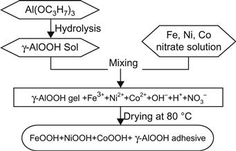
Figure 5.14 shows an example of a sol–gel method using an organic method (aluminum isopropoxide) to prepare the nanocomposite particles Ni65Fe31Co4/Al2O3.
Chemical codeposition treatment depends on the codeposition of metal ions in the solution through a chemical reaction. First, metal salts are prepared with a good proportion and mixed evenly in the solution, followed by using alkali as the precipitating agent to achieve codeposition of a variety of metal ions.
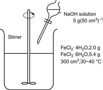
Figure 5.15 shows Fe3O4 nanoparticles prepared by codeposition. Chloride solutions with divalent iron ions and trivalent iron ions are deposited under the action of the alkali sodium hydroxide.
In MOCVD, the evaporated metal organic matter is mixed and introduced into a vacuum chamber. Under the effect of the heat, the gas-phase reaction is induced to promote the decomposition of organic matter to form metal nanoparticles or thin films. In the presence of oxygen, metal oxides can be formed. Commonly used metal organic compounds are M-(tmhd) 2,3 M-(thd), and others, and the organic part of 3 M-(thd) is a 4-methyl-G flavanone.
5.4.2.5 Preparation of Magnetic Nanoparticles in the Magnetic Fluid
Preparation of magnetic fluids involves the full use of the nanoparticle surface effect, namely adsorption and variation of surface composition. Long chains, such as the hydrophilic carboxyl-COOH in fatty acids, are adsorbed on the surface of magnetic nanoparticles, whereas the lipophilic alkyl CnH2n+1 is linked with the base magnetic fluid, such as polyphenylene ether, which acts as surfactant. Typical surfactants include oleic acid, polyimide, polyethylene amine, and others.
5.4.2.6 Two-Dimensional Nanowire Array: Template Method
Preparation of a high-quality template is a prerequisite for this approach. Commonly used templates are polymer, nanotube, molecular, porous alumina film, reverse micelle, block copolymer, and life body template.
1. Polymer track etched template
Nuclear irradiation of the fission fragment can produce traumatic pits in a polymer polyester or polycarbonate film, and then it is chemically treated to form a random distribution of cylindrical nanotemplates with uniform diameter. The minimum diameter of these templates is 10 nm. However, they are divergent because of nuclear radiation and cannot guarantee that the hole is vertical to the template surface.
2. Zeolite-type ordered template
As mentioned, the surfactant polymer is hydrophilic at one end and lipophilic at the other. When added to the solution with inorganic precursors, the lipophilic end will float to the surface because of the exclusion of water. With the increase of surfactant concentration, the lipophilic side floating to the surface will be saturated, followed only by assembly into micelles within solution. The lipophilic side is the inner side, with the hydrophilic outer side reducing the energy. Micelles can be formed in spherical, columnar, and laminar periodic arrangements. The space between micelles is surrounded by the solution with inorganic precursors. After this, the drying treatment is used to remove the solution water, which is heated to burn off the organic matter, forming the mesoporous molecular sieves composed of the inorganic wall. This process is also used as a template.
3. Carbon nanotube template method
Carbon nanotube itself as the carbon source can take part in the reaction forming one-dimensional solid nanowires with a basic shape of the original carbon nanotube. This method is still not used for preparation of magnetic nanowires.
4. The second anodization to prepare the Al2O3 template
High-purity aluminum chips with thickness of 0.5 mm or less are treated with 2 h of 500-degree vacuum annealing, followed by electrochemical polishing. In the H2SO4 or H2C2O4 electrolyte, these chip electrodes undergo anodic oxidation at constant temperature and pressure for more than 10 hours. In a mixture of 6 wt% H2PO4 and 1.8 wt% H2CrO4, the formed oxide film can be completely dissolved. Under the same conditions, these aluminum chips are given a second anodic oxidation of 2–4 h to obtain the template as shown in Figures 5.16 and 5.17.
5. Double-pass template
If the remaining aluminum is removed from the template in a mixture of 20% HCl and 0.1 M CuCl2, followed by use of 5 wt% H2PO4 to remove the dense alumina barrier layer at the bottom, then a double-pass template can be obtained as shown in Figure 5.18.
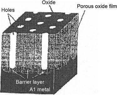
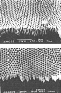
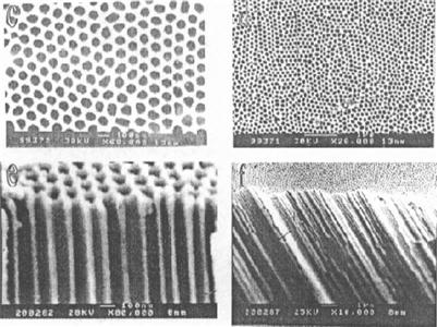
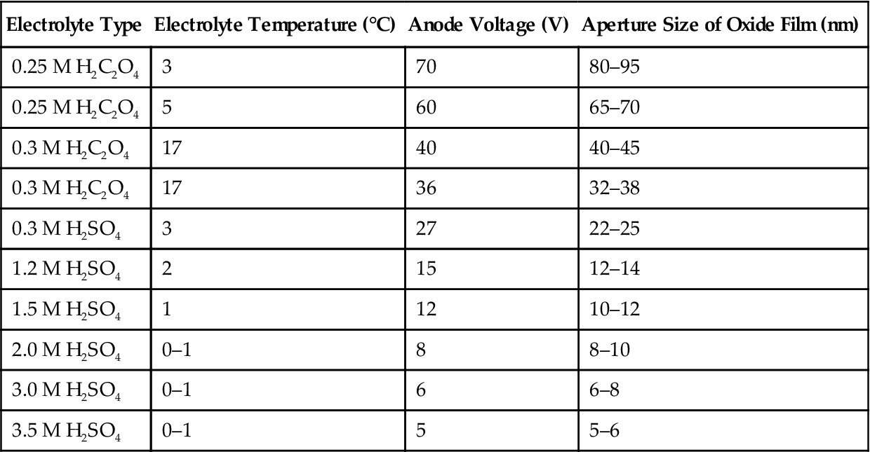
Table 5.9 shows a condition for the actual control of pore size.
Table 5.9
Conditions for Preparation and the Aperture Size of the Template of the Synthesized Al2O3 Ordered Array
| Electrolyte Type | Electrolyte Temperature (°C) | Anode Voltage (V) | Aperture Size of Oxide Film (nm) |
| 0.25 M H2C2O4 | 3 | 70 | 80–95 |
| 0.25 M H2C2O4 | 5 | 60 | 65–70 |
| 0.3 M H2C2O4 | 17 | 40 | 40–45 |
| 0.3 M H2C2O4 | 17 | 36 | 32–38 |
| 0.3 M H2SO4 | 3 | 27 | 22–25 |
| 1.2 M H2SO4 | 2 | 15 | 12–14 |
| 1.5 M H2SO4 | 1 | 12 | 10–12 |
| 2.0 M H2SO4 | 0–1 | 8 | 8–10 |
| 3.0 M H2SO4 | 0–1 | 6 | 6–8 |
| 3.5 M H2SO4 | 0–1 | 5 | 5–6 |
We can see from Figure 5.18 that the Al2O3 template generally self-assembles as a hexagonal close-packed ordered array, and its mechanism can be summarized as follows. In the initial oxidation, a dense oxide layer (barrier layer) is formed while maintaining the same thickness under certain conditions. Then, anodic oxidation depends on ion diffusion in the electric field. Because the volume of alumina is greater than the volume of aluminum, a thick oxide layer may expand inside and produce large stress. In the common effect of electric field, stress, and acidic medium, weak spots of oxide film may experience destruction of selective dissolution to form a porous structure. Uniformity of the role of stress results in the lowest energy because the holes are self-assembled in a hexagonal close-packed ordered array.
With the template method, it is easy to control the scale and uniformity of nanowires to facilitate preparation of nanoarrays. Nonetheless, nanowires prepared in this way mostly have polycrystalline structures. Furthermore, nanowires are prone to damage when the template is removed. In addition, several of the aforementioned manufacturing methods are apparently difficult to apply in industrial production. Designing a new preparation method is an important creation itself. Many important materials are actually discovered when researchers try to devise new preparation methods. The description in this section is only an introduction and aims to initiate work that should be based on open ideas and innovations.
5.5 GMR Materials
5.5.1 GMR Effect and Applications [9]
While moving in a material, electrons may be affected by the cations brought about by the lattice atoms or the impure atoms, so their motion path may change and therefore they may collide with these lattice atoms, producing some heat; such a process is called the “resistance effect.” In summary, the resistance effect is the result of the lattice hindering the motion of electrons. If the movement of electrons in materials is applied with a magnetic field, it will increase the probability of electron collisions with the cations, that is, it will lead to increased resistance. Because resistance is changed as a result of the impact of the magnetic field or a magnetic role, it is called magnetoresistance to differentiate from general resistance properties. In other words, magnetoresistance refers to the change in a particular magnetic field. Generally, both magnetic metal and alloy may accompany the magnetoresistance phenomenon, usually described by the rate of resistance change Δρ/ρ (or ΔR/R![]() ). Common metal conductors have a very small Δρ/ρ, which is only approximately 10−5%. For a magnetic metal or alloy material (for example, Permalloy), Δρ/ρ may be up to 3–5%.
). Common metal conductors have a very small Δρ/ρ, which is only approximately 10−5%. For a magnetic metal or alloy material (for example, Permalloy), Δρ/ρ may be up to 3–5%.
The so-called GRM effect manifests itself as a significant decrease in electrical resistance in the presence of a magnetic field. Such a decrease is usually 10 times that of the magnetoresistance values that may occur in magnetic metals and alloys.
In 1986, the German science team of Grunberg made an important discovery in Fe/Cr/Fe three-layer film: the chromium layer between two iron layers can produce coupling.
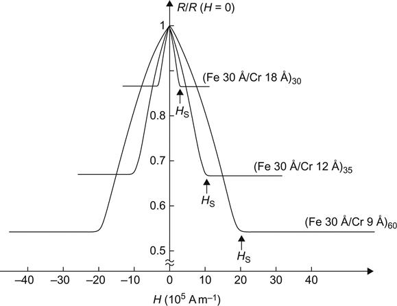
In 1988, Kent’s research team at Paris University, France, first observed the GMR effect in [Fe/Cr] periodic multilayer films. When applied with an external magnetic field, its resistance decreased, presenting a rate of change up to 50% (Figure 5.19), so it is called the GMR effect. This discovery elicited great interest in the international science community.
In the 1990s, Fe/Ag, Fe/Al, Fe/Au, Co/Cu, Co/Ag, and Co/Au nanostructured multilayer films were found to have characteristics of GMR. In 1995, researchers used an Al2O3 insulating layer instead of the conductor Cr and observed the phenomena of large TMR.
Based on the discovery of GMR and TMR, a new branch of the discipline—magnetic electronics—is gradually taking shape.
From then on, scientists have been engaged in persistent efforts to transform the discovery into industrialization of the innovative information technology. IBM, in 1994, developed a read head with a giant magnetoresistive effect, increasing the disk recording density by 17-fold, and magnetic disks are again leading in the competition of recording density with CD-ROMs. The application of GMR heads led to rapid developments in the computer industry, breaking the bottleneck in the transmission and storage of images on the information superhighway. At present, the storage density has been as high as 56 GB/in.2. GMR heads help generate a total of US$40 billion annually in the world market. Moreover, Motorola announced that it had successfully developed a GMR magnetic random access memory in 2001, which implies a market capacity of US$100 billion.
By using the GMR effect with different resistance characteristics in different magnetic states, magnetic random access memory (MRAM) can be made to retain information in the absence of power supply.
In 1999, a hard disk drive that used GMR heads (HDD) began to be sold, with a storage density up to 11 Gbits/in.2. In 1990, this figure was merely 0.1 Gbits/in.2, so the increase in one decade is 100-fold.
At present, research and development of GMR are booming, but the study commenced with respect to the aforementioned TMR multilayer films applied in the novel random access memory (MRAM). Based on the spin polarization effect, the spin transistor has also been suggested.
5.5.2 Classification and Comparison of Magnetic Resistance
In terms of the magnetic materials that have been studied, the magnetoresistance effect can be divided into ordinary magnetoresistance (OMR), technical magnetization-associated anisotropy magnetoresistance (AMR), GMR specific to magnetic multilayers and particulate film, colossal magnetoresistance (CMR) doped with rare earth oxides, and TMR. To understand the nature of the magnetoresistance, we must first understand the principle of electron scattering.
Electron scattering plays a fundamental role in all transport processes. In an ideal cycle field where rules of atom array are completely ordered, the electrons will be in a determining k-state and transition does not occur. But in reality, atoms do not statically remain in the grid points. Because of thermal vibrations, atoms often deviate from the grid points, which can be regarded as a perturbation of periodic potential field to cause electronic transitions known as lattice scattering. The size of the lattice scattering is proportional to the electron density of energy states on the Fermi side. In addition, the material impurities and defects also undermine the periodic potential field, resulting in electron scattering.
For a general nonmagnetic metal, the electron spin is degenerated without any net magnetic moment. And the electronic states in the vicinity of the Fermi surface, of course, are exactly the same as for the spin-up and spin-down. Thus, in transport processes, the electron flow is nonspin-polarized.
With a common nonmagnetic metal, electron scattering is mainly in the state of spin degeneracy between s electrons, showing a larger mean free path of electrons. With the Drude theorem σ=ne2τ/m, it can be very easy to estimate that good metal conductors may have a mean free path of approximately 100 Å.
Unlike s electron scattering in ordinary metals, ferromagnetic metals, such as iron, cobalt, and nickel, feature the existence of s electrons and d electrons with great density of states at the Fermi surface. In the transport process, conduction electrons are expected to endure s–d scattering that is much higher than the s electron scattering, so the conduction electron here has a much smaller mean free path.
Because the spin-up 3d subband (more in spin) and spin-down 3d subband (few in spin) are not equal in density of states on the Fermi surface, the size of scattering will not be the same as that of the conduction electrons in a different spin mode. Therefore, the spin-up electrons may have a different mean free path (λ↑) from that of the spin-down electrons (λ↓).
Based on the theoretical and experimental evidence, the transport process of ferromagnetic metals or alloys can be decomposed into spin-up and spin-down channels of electronic conductivity, which have parallel connection and are almost independent of each other. This is a two-fluid model of spin-dependent scattering.
A normal magnetoresistance effect is common to all magnetic and nonmagnetic materials. Lorentz force from the magnetic field on the carrier can cause deviation from the motion of conduction electrons in space or the occurrence of spiral motion to increase the probability of electron impact and resistance; therefore, MR is always positive.
MR changes in magnetic conductors are associated with magnetic fields and the angle between the directions of current in the conductor, for example anisotropy, known as anisotropic magnetoresistance. When the external magnetic field is applied in a direction either parallel or perpendicular to the direction of the current, the resistivities ρ//![]() and ρ⊥
and ρ⊥![]() of anisotropic magnetic material are different from each other. Usually, Δρ/ρ0=(ρ//−ρ⊥)/ρ0
of anisotropic magnetic material are different from each other. Usually, Δρ/ρ0=(ρ//−ρ⊥)/ρ0![]() , which is used to evaluate the size of the anisotropic magnetoresistance. Here, ρ0
, which is used to evaluate the size of the anisotropic magnetoresistance. Here, ρ0![]() is the magnetic resistivity in the ideal annealing state. A commonly used AMR material highly sensitive to magnetic fields is Permalloy (Ni80Fe20). At room temperature, its magnetoresistance change rate is 5%. In ferromagnetic metals, the AMR effect is strongly dependent on the direction of spontaneous magnetization. It is caused by the motion from anisotropy of the ferromagnetic domain in an outer magnetic field. In fact, this magnetoresistance corresponds to the technical magnetization, that is, the corresponding resistance changes from the demagnetization state to the process toward magnetic saturation. The zero-field resistivity is also associated with its history. In ferromagnetic materials, the anisotropic magnetoresistance effect comes from the anisotropic scattering, that is, it is derived from the spin-orbit coupling, which may reduce the symmetry of electron wave functions so that electron spin and its track are associated with each other.
is the magnetic resistivity in the ideal annealing state. A commonly used AMR material highly sensitive to magnetic fields is Permalloy (Ni80Fe20). At room temperature, its magnetoresistance change rate is 5%. In ferromagnetic metals, the AMR effect is strongly dependent on the direction of spontaneous magnetization. It is caused by the motion from anisotropy of the ferromagnetic domain in an outer magnetic field. In fact, this magnetoresistance corresponds to the technical magnetization, that is, the corresponding resistance changes from the demagnetization state to the process toward magnetic saturation. The zero-field resistivity is also associated with its history. In ferromagnetic materials, the anisotropic magnetoresistance effect comes from the anisotropic scattering, that is, it is derived from the spin-orbit coupling, which may reduce the symmetry of electron wave functions so that electron spin and its track are associated with each other.
In the past it was difficult to produce high-quality nanoscale samples. By the 1980s, however, because of the liberation from these restrictions, metallic superlattices have become a research frontier that has attracted the interest of many researchers. The researchers of condensed matter physics have been performing a wide range of basic research on the nature of such artificial materials, including magnetic ordering, interlayer coupling, electron transport, and quantum confinement.
Magnetic multilayers are a multilayer film system resulting from the alternately repeated growth of nanoscale ferromagnetic films (Fe, Co, Ni, and its alloys) and nonmagnetic films (including 3d, 4d, and 5d nonmagnetic metal). A combination of contemporary mesoscopic magnetism, nanomagnetic materials, and nanotechnology, it is developed as a kind of artificial superlattice magnetic material with unique magnetic properties. In 1988, when a single crystal (100) Fe/Cr/Fe three-layer film grew from MBE with a Cr layer thickness of 9 Å (at 4.2 K or below) and a 20 kOe external magnetic field, it showed a value of magnetoresistance of MR (%)=Δρ/ρs=(ρ(H)−ρs)/ρs, up to 100%, and it is called the GMR effect.
With the sputtering process, Parkin and colleagues prepared multicrystalline Fe/Cr/Fe three-layer film and (Fe/Cr) multilayers also displayed the GMR effect. The MR values of the latter are 25% and 110% at room temperature and the low temperature of 4.2 K respectively.
Subsequently, research discovered that many magnetic multilayers, which constitute the alternative growth of a variety of iron magnetospheres (Fe, Ni, Co, and its alloys) and nonmagnetic layers, had a GMR effect, especially the polycrystalline (Co/Cu) multilayer films. Their GMR values were 130% and 70% at the low temperature (4.2 K) and room temperature respectively, and the added saturation field was approximately 10 kOe.
In artificial magnetic metal films with nanostructures, there is another essential material in addition to superlattices and multilayers: the granular film. It is a composite film formed by microparticles embedded in mutually nonsolutionable films. It has the double features of microparticles and thin film and their interaction effects. In principle, if any two elements are not soluble in equilibrium conditions, then either the co-sputtering or co-evaporation process can be used to prepare granular films. Therefore, research on the magnetic GMR effect is necessary in terms of its extension from magnetic multilayer films to granular films.
In 1992, Co–Cu and Co–Ag granular films were found to have a GMR effect similar to that in multilayer films. Subsequent work focused on two types of granular films comprising Fe, Co, and Ni metals and alloys based on Cu and Ag. Among the granule films that may produce the greatest GMR effect, the share of iron group elements in the volume has a percentage of approximately 15–25%, which is below the percolation threshold to form a network structure. At this time, iron group elements were embedded in thin films mainly in the form of microparticles, and the best size of microparticles is in the range of several nanometers to 10 nm, so that ferromagnetic particles of such sizes are usually in a superparamagnetic state at room temperature.
As with multilayer films, theoretically the GMR effect of granular films is associated with spin-dependent scattering and particularly with interface scattering. Theory suggests that the GMR effect of granular films is inversely proportional to the diameter of magnetic particles; for example, it is proportional to the specific surface area of the particles. Particles are usually randomly distributed in the films, and most of the conduction electrons are transmitted through the particles, similar to the case of multilayer film CPP (current perpendicular to it). So, a larger GMR effect can be easily obtained in granular films. However, there is a problem. Because of the ferromagnetic particles in a superparamagnetic state, the access of GMR usually requires a very high saturation field.
A magnetic tunnel junction has a sandwich structure, which is constituted by a ferromagnetic film, an insulator film, and a ferromagnetic thin film. The magnetoresistance phenomenon that corresponds to the tunnel junction is known as the TMR.
The TMR comes from the asymmetry between two ferromagnetic layers on the density of states of the spin-up and spin-down electrons. Assuming there is no spin-flip scattering (the spin conservation of electrons in tunneling process), the probability of spin polarization depends on the relative orientation of magnetization in two ferromagnetic layers. When the magnetizations are parallel to each other, the majority of electrons share the same spin orientation in the energy band of two ferromagnetic materials. The number of states that can be filled is maximized in the matching degree in the vicinity of a Fermi surface, creating the largest tunneling current and the smallest tunneling resistance. In contrast, in antiparallel magnetization, electron tunneling occurs between the majority of electronic states in a ferromagnetic layer and a few electronic states in the other ferromagnetic layer. This mismatch between densities of states results in the smallest tunneling current and the largest resistance. Because the external magnetic field is applied so that magnetization changes from parallel to antiparallel, or vice versa, the magnetoresistance phenomenon may occur. Because electron transport in a magnetic tunnel junction is based on the mechanism of the tunnel effect, it is called TMR.
TMR has the advantages of a small saturation field and high field sensitivity. In the magnetic tunnel valve, the magnetic field that has overcome two-layer ferromagnetic coercivity can subsequently have its magnetization directions transferred to be parallel with the direction of the magnetic field. At this time, tunnel resistance tends to have a very small value. If the magnetic field is reduced to a negative value, then the ferromagnetic field with the smaller coercivity will first reverse the magnetization direction. The two ferromagnetic layers are placed in the opposite direction of magnetization, making the tunnel resistance very high. Thus, only a very small external magnetic field can lead to a maximum value of TMR, so TMR is very high in magnetic field sensitivity. Miyazaki produced Fe/Al2O3/Fe magnetic field sensitivity of 8%/Oe; Moodera and associates obtained CoFe/Al2O3/Co sensitivity of 5%/Oe. Both showed results that are well beyond those of multilayer GMR and the oxides CMR. For resistance in the magnetic tunnel junction under zero field, the thickness of the insulating layer can be adjusted to change the number of orders of magnitude, but the TMR value is not changed. Meanwhile, changing their own resistances of multilayer films and metal oxides under the zero field is not as easy as it looks. Therefore, TMR can be used to make controllable high-resistance junctions.
5.5.3 Physical Mechanism of GMR
5.5.3.1 Magnetic Exchange Coupling
Two layers of ferromagnetic thin films separated by a layer of nonmagnetic metal thin film may have magnetic exchange coupling in between, from which the GMR effect occurs. Magnetic exchange coupling and GMR effect may have periodic oscillations depending on the nonmagnetic film thickness.
In the Fe/Cr/Fe system, the coupling state exists between adjacent iron layers. With the increase of the Cr layer thickness, coupled oscillation will be attenuated in the form of alternating positive and negative states. This makes the magnetic moments of adjacent Fe layers alternate from an antiparallel orientation with each other to a parallel orientation (Figure 5.20). In the outer magnetic field, the iron magnetosphere in multilayer films will also change in the antiparallel magnetization state. When electrified with current, this change in magnetic state is reflected in changes in the form of resistance. This is the physical mechanism of the GMR phenomenon.
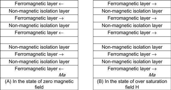
The coupling between iron layers with the Cr electrons as an intermediary may have an oscillation attenuation as the Cr layer thickness increases. The average scope is 1–3 nm, which limits the Cr layer thickness. The electronic mean free path (10–20 nm) and the spin diffusion length (30–60 nm) are both very short for metals, especially magnetic metals. This constitutes a further restriction on the individual sublayer thickness of multilayer films.
For these reasons, we can say that GMR and TMR studies depend entirely on the progress of nanomaterials science. No innovation or transformation can be made without this basis. However, the nanoscale is so tiny that it brings a challenge in the preparation of multilayer films and their microstructural characterization.
5.5.3.2 GMR Effects of Metal Superlattice
At present, it is well known that metallic superlattices to produce the GMR effect are required to satisfy the following three conditions. First, the system can change the magnetization state in the outer magnetic field. For example, in ferromagnetic conductor/nonmagnetic conductor superlattices, an antiparallel spin structure can constitute a zero magnetic field (Figure 5.20A) and can become a parallel spin structure when the external magnetic field is higher than magnetic saturation (Figure 5.20B). Second, metal superlattices should have a shorter cycle than the mean free path of the carrier electron. Third, the two kinds of electronics that differ in spin orientation (up or down) must be strikingly different in scattering on magnetic atoms.
Magnetoresistance phenomena were discovered as early as 1856, but an explanation was not available until the establishment of quantum theory. To tackle the problem of noninteger magnetic distance in ferromagnetic transition metals, Stoner proposed the band-splitting exchange model. Because of the exchange interaction, the d electronic band that contributes to the magnetic distance may split, causing the spin-up electronic energy bands to come down below the Fermi level. Therefore, the number of spin-down electrons is less than the number of spin-up electrons. The difference between the two caused the problem of noninteger magnetic distance in ferromagnetic transition metal elements (Figure 5.21). Inspired by this model, Mott proposed his famous two-fluid model. He indicated that in ferromagnetic metals, the conductive s electron is affected by the scattering from the magnetic distance of magnetic atoms (i.e., the role of local d electrons), and the scattering probability depends on the relative orientation of the spin direction of conductive electrons and the direction of the magnetic distance of magnetic atoms in solids. Based on this, a theoretical model of the GMR effect can be established. The following is a brief introduction of how the two-fluid model is used to explain the GMR effect.
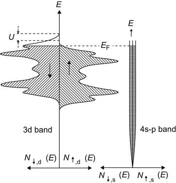
Magnetic metallic multilayers have nothing to do with the direction of the magnetic field in terms of the GMR effect, which only depends on the relative orientation of magnetic moments in adjacent ferromagnetic layers. The role of the external magnetic field is to change the relative orientation. This shows that electron transport is associated with electron spin scattering.
In s–d scattering associated with the spin, when the electron spin is parallel to the spin-up 3d subband (i.e., the majority in spin) in ferromagnetic metals, the average free path is longer and combined with a lower corresponding resistivity; when the electron spin is parallel to the spin-down 3d subband (i.e., antiparallel to the majority in spin) in ferromagnetic metals, the average free path is shorter and the corresponding resistivity is higher. Therefore, as antiferromagnetic coupling occurs in magnetic moments between neighboring ferromagnetic layers, electrons subject to weak scattering in a ferromagnetic layer must face strong scattering after entering into another ferromagnetic layer. As a whole, all electrons have strong scattering. If and when the magnetic moments of the adjacent ferromagnetic layer tend to be parallel under the influence of the magnetic field, the spin-up electrons will suffer weaker scattering in all the magnetospheres, equivalent to the spin-up electrons that have a short-circuit state. This is a simple interpretation based on Mott’s two-fluid model of the GMR effect. This process can be demonstrated with a simple resistor network (Figure 5.22). That is, if the magnetic moments in adjacent magnetic layers are in an antiparallel arrangement, then the resistor network is in a high-impedance state, and if a magnetic field is larger, with magnetic moments in adjacent magnetic layers in a parallel arrangement, then the resistor network would be in a low-impedance state.
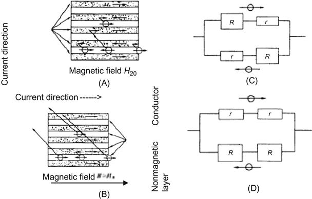
5.5.4 GMR Biosensors [10–13]
The GMR effect has great potential. With external magnetic fields, the GMR effect may lead to reversal of the magnetic moment to trigger resistance mutations and, further, to the formation of a switching effect on magnetic power conversion. This makes GMR a possible candidate for computer read heads and, thus, a candidate to greatly improve the storage density of computers. Magnetoresistance and GMR read heads are designed to meet the needs of computers, multimedia, and the information superhighway for the development of high density, large capacity, and miniaturization. It is the key technology and an effective way to achieve new ultrahigh-density magnetic recordings. At present, a breakthrough has been achieved in improving the computer’s storage density. GMR multilayers have been reported to be able to achieve readout heads of 22 GB/in.2. GMR heads for hard disks have already been applied and 10–100 Mb of 3-in. disks will become a reality within a few years.
GMR can also be applied to high-sensitivity magnetic sensors, various types of motion sensors, and giant MRAM. In mechanical and electrical automation, automotive, and aerospace industries, GMR has also shown its wide range of application. Highlighted here is the description of GMR biosensors.
5.5.4.1 Introduction of Biosensors
Biosensors comprise a very active research and engineering field. Together with bioinformatics, biochips, biocybernetics, bionics, biology, and computer disciplines, it is a subject that combines life science and information science. Their common aims and features are: to explore and reveal the basic rules of production, storage, transmission, processing, conversion, and control of information in living systems; and to explore the application of the basic methods for human economic activity. Priorities in the research on biosensor technology include extensive application of bioactive materials and sensor integration and research and development of the transducers with recognition functions. In addition, biosensor technology is used to develop itself into the original technology in the manufacture of novel analytical instruments and analysis methods, with a particular focus on the research and development of their applications. A wide range of material objects with biological activity are applicable in biosensors, including biological macromolecules, cells, organelles, tissues, and organs, as well as synthetic molecularly imprinted polymers. Because the study of molecular DNA or protein molecule identification technology has become an independent field (biochips, i.e., DNA chips, protein chips), we do not discuss these areas in detail in this book.
Biosensor research originated in the 1960s. In 1967, Updike and Hicks made the first biological sensor by assembling the immobilized film and oxygen electrode of glucose oxidase, namely the glucose enzyme electrode. By the 1980s, the field of biosensor research had been basically formed. Since then, biosensors, including enzyme sensors, have gradually flourished. Biosensors, starting with one or more enzymes as molecular recognition elements, have been developed with the design of other biological molecules for identification components, for example enzyme–substrate, enzyme–coenzyme, antigen–antibodies, hormone–receptor, and molecules with DNA double-helix structures. One side is immobilized and may be used as a molecular recognition element to choose and measure the other. Apart from biological macromolecules, components with the recognition of certain environmental components, such as organelles, cells, tissues, and microorganisms, can also be candidates for the recognition element. Even synthetic receptor molecules and sensors can be combined to determine microorganisms, cells, and associated biological molecules.
Sensors combined with bioactive materials can be various types of physical or chemical sensors, such as electrochemical (potential measurement, conductivity measurement, impedance measurement), optical (photoluminescence, surface plasmon resonance), machinery (lever, pressure electric reaction), heat (thermal resistance), or electricity (ion or enzyme field-effect transistor). All of these combinations with biometric identification features are known as biosensors.
The 9/11 terrorist attacks in the United States were the beginning of mass terrorist activities by international terrorists. However, the aftermath of this human tragedy caused by terrorism is far from over. Biological weapons might be the most dangerous means of terrorist attacks. The danger lies not only in its immediate effect but also in the long-lasting potential threat it poses. Because there is an incubation period from committing crime involving biological weapons to the early symptoms of diseases that will have been detected, a serious pandemic disease caused during a short latent period may pose a great threat to social stability and security. Therefore, bioterrorism defense has been given the top priority in today’s fight against terrorism by the international community. It is a very complex task that requires long term and arduous efforts. The need to prevent bioterrorism attacks has stimulated to some extent the research and development of biological sensors and detectors.
5.5.4.2 GMR Sensor Chip
The GMR sensor chip is a class of devices that mainly make use of magnetic nanometallic multilayer thin films with the GMR effect, which is compatible with semiconductor integrated circuits through the integration process. Since the discovery of the GMR effect, manufacturers and academia in various countries have attached great importance to it, making it quite popular in condensed matter physics.
The in-depth research and development and use of the GMR effect have opened a window to the gradual emergence of the spin-up subdiscipline. This is a novel discipline mainly aimed at research on the role of electron spin and the development of special purpose devices at the same time. The National Science Foundation claimed that the development and application of a spin subdiscipline will herald the arrival of the fourth industrial revolution.
Giant magneto-impedance materials are highly sensitive to magnetic fields (in the case of low-frequency magnetic induction and high-frequency magneto-impedance, a value up to 1,000%/Oe has been reported, and only a few Oe changes in external magnetic field are required). In addition, these materials feature high-temperature stability, small size, and low power consumption. In 1994, the United States first realized NVE’s GMR effect in mass production of giant magnetoresistive magnetic field sensors. Because of its high sensitivity, thermal stability, and GMR, sensor chips can easily supersede Hall and the magnetoresistance (AMR) components, it is widely used in information, electrical, electronic power, energy management, automotive, magnetic information read–write, and industrial automation fields, among others.
5.5.4.3 GMR Biosensors
Considerable progress has been made regarding the current research on using magnetic particles as magnetic markers for detection of biological samples. Compared with other markers, such as conventional fluorescent markers, magnetic markers have many potential advantages. First, magnetic bead drops have very stable magnetic properties and can be used for repeated measurements because their magnetic properties will not be affected by chemical reagents and light. From the detection point of view, normally there is no strong magnetic background signal in samples of biological molecules. More importantly, the magnetic field is not shielded by water-based reagents or biological materials. Applied with a magnetic field, magnetic markers can achieve on-chip manipulation for molecular orientation or identification. Also, a strong magnetic field can be removed by analyzers with magnetic marker material to ensure the reuse of biochips.
GMR biosensors are commonly used in the detection of magnetic markers of biological samples. The new GMR biochip has several advantages. It is compatible with the IC process, biological information can be directly converted into electrical signals and subject to detection, and it is suitable for automated analysis. In addition, expensive high-precision optical measurement systems are not required. It can easily reduce or even eliminate background noise. It has high sensitivity and is expected to extract biological information from samples without undergoing PCR amplification. It is portable—a central laboratory is not required. Also, single-chip testing can be performed for multiflux.
GMR biosensors with magnetic markers work to identify biological molecules. First, the sample solution for testing and magnetic microspheres solution are mixed for reaction, whereby analyte molecules will complete the process of magnetic marking. Then, the marked sample solution is transported into the biomolecular recognition domain on the GMR biosensors, which are bound with a known specific receptor that is able to complete the specific combination with the corresponding target molecules. If the marked sample solution contains the target molecules that can be specifically combined with the known receptor bound on GMR biosensors, then a combination of both will remove the sample uncombined. GMR biosensors will detect the magnetic field signal produced by the micro-touch balls marked on target molecules to achieve the purpose of biomolecular recognition.
Until now, there have been reports of a variety of GMR biosensors used to perform testing on biological samples with magnetic markers. Romanian scientists have also developed a GMR biosensor that can detect biological samples based on the magnetic markers. Under the effect of the outer magnetic field, magnetic particles may come close to the giant magneto-impedance microfilaments, causing changes in magneto-impedance of microfilaments. By measuring this change, we can understand the distribution of magnetic particles in solution. Because they are adhesive with objective molecules, the distribution of target molecules is available in solution. The range of application of this method can be further expanded with its sensing function in biological or medical testing of antibodies and biological specimens.
Researchers at Stanford University collaborated with the Genome Technology Center in the development of a magnetic biochip through integrated GMR of a high-density biosensor array with the standard CMOS chip. They used a “multipartition” array structure, whereby each biological sample point was consolidated with several sensor pixels to improve the sensitivity of low-concentration samples. Marked with labels to magnetic bead for biological molecules, HD-based technologies, such as GMR, can produce gene chips without using conventional fluorescence detection. This makes it possible to detect DNA hybridization at low cost. One way is to separate the DNA family to match the target DNA attached onto the chip surface of GMR sensors. Target DNA in solution, which is surrounded by the GMR sensors, hybridizes with matching DNA on the chip. Then, DNA with nanomagnetic labels is partially hybridized with the naked target DNA. As a result, magnetic labels are selectively attached to the chip surface. The GMR sensors can detect the amount of nanomagnetic tags attached, which combines biological molecules, cells, and bacteria. Unlike the complex and expensive optical detection systems, GMR biochip measurement of electrical signals comes directly from the sensors, making it a realistic candidate for a highly portable DNA detecting device.
Researchers have designed and manufactured biochips that contain 1,008 sensors within 1 mm2. Such a device also has low noise and high-throughput readout channels for high-sensitivity DNA detection.
Another type of GMR biosensor is the so-called bead array counter (BARC). The development of GMR materials creates high-quality materials for highly sensitive magnetic sensors. This is the fundamental reason why BARC has boomed in recent years. However, the development of BARC is inseparable from the development of magnetic bead drops. They must be made with superparamagnetic materials—that is, the magnetic features are evident only when there is a magnetic field. The general magnetic bead droplets comprise a nucleus and a cladding layer, where the nucleus is iron oxide and the cladding layer is generally made of high polymers attached to proteins or antibodies.
As a DNA probe is based on the magnetic field rather than the optical and fluorescence features, BARC is composed of a linear magnetic field sensor array (Figure 5.23). Each microsensor is coated with a special DNA test agent that matches with a microbial genome in biological weapons. When the microbial DNA samples encounter the testing DNA probe, a single drop of the magnetic beads will be formed. When a sensor encounters a magnetic bead, the sensor’s resistance will decrease. Although the decrease is very small, it can be detected. The more bead drops comprising a biosensor, the greater the resistance variation will be.
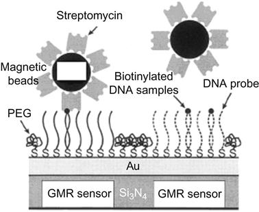
At present, biochips have found their largest application in the areas of biological research and disease diagnosis. Although they have enormous potential, there are some key factors that prevent them from large-scale application. First, biochip analysis involves too many steps that require well-trained professionals. Second, the biochip testing process depends on very expensive biochemical and optical testing equipment. Such devices are not only costly but also need to be implemented in a large central laboratory. Despite these disadvantages, this novel device, by replacing traditional fluorescent markers with magnetic nanoparticles and using GMR sensors to detect biological information, has a bright future.