
chapter 4
Testing the Factorial
Validity of Scores From
a Measuring Instrument
First-Order Confirmatory
Factor Analysis Model
For our second application, we once again examine a first-order confirmatory factor analysis (CFA) model. However, this time we test hypotheses bearing on a single measuring instrument, the Maslach Burnout Inventory (MBI; Maslach & Jackson, 1981, 1986), designed to measure three dimensions of burnout, which the authors labeled Emotional Exhaustion (EE), Depersonalization (DP), and Reduced Personal Accomplishment (PA). The term burnout denotes the inability to function effectively in one's job as a consequence of prolonged and extensive job-related stress: “Emotional exhaustion represents feelings of fatigue that develop as one's energies become drained”; “depersonalization,” the development of negative and uncaring attitudes toward others; and “reduced personal accomplishment,” a deterioration of self-confidence and dissatisfaction in one's achievements.
Purposes of the original study (Byrne, 1994a), from which this example is taken, were to test for the validity and invariance of factorial structure within and across gender for elementary and secondary teachers. For the purposes of this chapter, however, only analyses bearing on the factorial validity of the MBI for a calibration sample of elementary male teachers (n = 372) are of interest.
CFA of a measuring instrument is most appropriately applied to measures that have been fully developed, and their factor structures validated. The legitimacy of CFA application, of course, is tied to its conceptual rationale as a hypothesis-testing approach to data analysis. That is to say, based on theory, empirical research, or a combination of both, the researcher postulates a model and then tests for its validity given the sample data. Thus, the application of CFA procedures to assessment instruments that are still in the initial stages of development represents a serious misuse of this analytic strategy. In testing for the validity of factorial structure for an assessment measure, the researcher seeks to determine the extent to which items designed to measure a particular factor (i.e., latent construct) actually do so. In general, subscales of a measuring instrument are considered to represent the factors; all items comprising a particular subscale are therefore expected to load onto their related factor.
Given that the MBI has been commercially marketed since 1981, is the most widely used measure of occupational burnout, and has undergone substantial testing of its psychometric properties over the years (see, e.g., Byrne, 1991, 1993, 1994b), it most certainly qualifies as a candidate for CFA research. Interestingly, until my 1991 study of the MBI, virtually all previous factor analytic work had been based on only exploratory procedures. We turn now to a description of this assessment instrument.
The Measuring Instrument Under Study
The MBI is a 22-item instrument structured on a 7-point Likert-type scale that ranges from 0 (feeling has never been experienced) to 6 (feeling experienced daily). It is composed of three subscales, each measuring one facet of burnout: The EE subscale comprises nine items, the DP subscale five, and the PA subscale eight. The original version of the MBI (Maslach & Jackson, 1981) was constructed from data based on samples of workers from a wide range of human service organizations. Subsequently, however, Maslach and Jackson (1986), in collaboration with Schwab, developed the Educators’ Survey (MBI Form Ed), a version of the instrument specifically designed for use with teachers. The MBI Form Ed parallels the original version of the MBI except for the modified wording of certain items to make them more appropriate to a teacher's work environment.
The Hypothesized Model
The CFA model of MBI structure hypothesizes a priori that (a) responses to the MBI can be explained by three factors: EE, DP, and PA; (b) each item has a nonzero loading on the burnout factor it was designed to measure, and zero loadings on all other factors; (c) the three factors are correlated; and (d) the residuals associated with each indicator item variable are uncorrelated. A schematic representation of this model is shown in Figure 4.1.1
An important aspect of the data to be used this chapter is that they are somewhat nonnormally distributed. That is to say, certain item scores on the MBI scale tend to exhibit kurtosis values that may be regarded as moderately high. Thus, before examining the Mplus input file related to the hypothesized model shown in Figure 4.1, I wish first to address the issue of nonnormality in structural equation modeling (SEM) and then outline how this problem can be addressed using Mplus. I begin with a brief overview of the nonnormality issue in SEM, followed by an overview of the MBI item scores with respect to evidence of nonnormality. Finally, I outline the approach taken by Mplus in the analyses of nonnormal data.
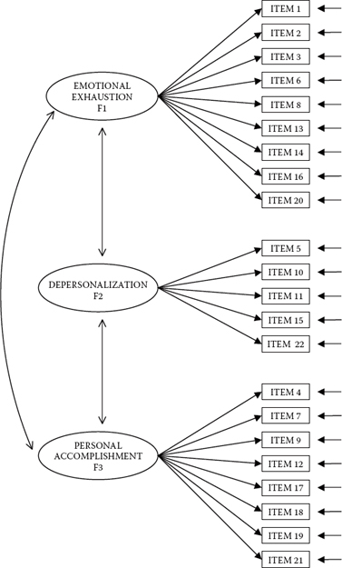
Figure 4.1. Hypothesized CFA model of factorial structure for the Maslach Burnout Inventory (MBI).
The Issue of Nonnormality in SEM
A critically important assumption in the conduct of SEM analyses is that the data are multivariate normal. This requirement is rooted in large sample theory from which the SEM methodology was spawned. Thus, before any analyses of data are undertaken, it is always important to check that this criterion has been met. Particularly problematic to SEM analyses are data that are multivariate kurtotic, the situation where the multivariate distribution of the observed variables has both tails and peaks that differ from those characteristic of a multivariate normal distribution (see Raykov & Marcoulides, 2000). More specifically, in the case of multivariate positive kurtosis, the distributions will exhibit peakedness together with heavy (or thick) tails; conversely, multivariate negative kurtosis will yield flat distributions with light tails (DeCarlo, 1997). To exemplify the most commonly found condition of multivariate kurtosis in SEM, let's take the case of a Likert-scaled questionnaire, for which responses to certain items result in the majority of respondents selecting the same scale point. For each of these items, the score distribution would be extremely peaked (i.e., leptokurtic); considered jointly, these particular items would reflect a multivariately positive kurtotic distribution. (For an elaboration of both uni-variate and multivariate kurtosis, readers are referred to DeCarlo, 1997.)
Prerequisite to the assessment of multivariate normality is the need to check for univariate normality, as the latter is a necessary, although not sufficient, condition for multivariate normality (DeCarlo, 1997). Research has shown that whereas skewness tends to impact tests of means, kurtosis severely affects tests of variances and covariances (DeCarlo, 1997). Given that SEM is based on the analysis of covariance structures, evidence of kurtosis is always of concern, in particular evidence of multivariate kurtosis as it is known to be exceptionally detrimental in SEM analyses.
Mplus, in contrast to other SEM programs (e.g., AMOS and EQS), does not provide a single measure of multivariate kurtosis. However, it does enable the provision of actual univariate skewness and kurtosis values. That Mplus does not yield a coefficient of multivariate kurtosis is moot and in no way detracts from its capacity or approach in dealing with the presence of such nonnormality in the data. Rather, the omission of this coefficient is simply in keeping with Muthén and Muthén's (2007–2010) contention that such representation based on a single number is both unnecessary and somewhat meaningless given the current availability of robust estimators today; as such, they recommend a comparison of both the scaled and unscaled χ2 statistics, as well as the parameter standard errors (Mplus Product Support, March 4, 2010).
Although it is possible to obtain values of skewness and kurtosis using Mplus, the process requires a greater understanding of the program notation than can be expected for my readers at this early stage of the book. To avoid much unnecessary confusion, then, I do not include these details here. However, for readers who may have an interest in knowing how to obtain observed variable skewness and kurtosis values using Mplus, I present this information via a walkthrough of the process in the addendum at the end of this chapter.
Based on other construct validity research bearing on the MBI (Byrne, 1991, 1993, 1994a), and as will be shown in Figure 4.8 in the addendum, it is evident that the data used in this application certainly exhibit evidence of kurtosis, an issue that must be addressed in our current analyses of MBI factorial structure.
In judging the extent to which kurtosis values may be indicative of nonnormality, we must first know the range of values expected in a normal distribution. Accordingly, when scores are normally distributed, the Standardized Kurtosis Index has a value of 3.00, with larger values representing positive kurtosis and lesser values representing negative kurtosis. However, computer programs typically rescale this value such that zero serves as the indicator of a normal distribution and its sign serves as the indicator of positive or negative kurtosis (DeCarlo, 1997; Kline, 2011; West, Finch, & Curran, 1995).
At this point, no doubt you are wondering how far a kurtosis value must deviate from zero before it can be regarded as problematic. Unfortunately, to date, there appears to be no clear consensus regarding this question (Kline, 2011) as absolute kurtosis values ranging from ± 2.0 (Boomsma & Hoogland, 2001; Muthén & Kaplan, 1985) to ± 7.0 (West et al., 1995) and higher (DeCarlo, 1997) have been proposed as possible early departure points of nonnormality. Thus, although kurtosis values may appear not to be excessive, they may nonetheless be sufficiently nonnormal to make interpretations based on the usual χ2 statistic, as well as the Comparative Fit Index (CFI), Tucker-Lewis Fit Index (TLI), and Root Mean Square Error of Approximation (RMSEA) indices, problematic. Thus, it is always best to err on the side of caution by taking this information into account.
In contrast to the lack of consensus regarding the point at which the onset of nonnormality can be considered to begin, there is strong consensus that when variables demonstrate substantial nonzero univariate kurtosis, they most certainly will not be multivariately normally distributed.
As such, the presence of kurtotic variables may be sufficient enough to render the distribution as multivariate nonnormal, thereby violating the underlying assumption of normality associated with the ML method of estimation. Violation of this assumption can seriously invalidate statistical hypothesis testing with the result that the normal theory test statistic (χ2) may not reflect an adequate evaluation of the model under study (Hu, Bentler, & Kano, 1992). (For an elaboration of other problems arising from the presence of nonnormal variables, readers are referred to Bentler, 2005; Curran, West, & Finch, 1996; West et al., 1995.) Although alternative estimation methods have been developed for use when the normality assumption does not hold (e.g., asymptotic distribution-free [ADF], elliptical, and heterogeneous kurtotic), Chou, Bentler, and Satorra (1991) and Hu et al. (1992) contended that it may be more appropriate to correct the test statistic, rather than use a different mode of estimation.
Indeed, Satorra and Bentler (1988) developed such a statistic that incorporates a scaling correction for the χ2 statistic (subsequently termed the Satorra-Bentler χ2, or S-Bχ2) when distributional assumptions are violated; its computation takes into account the model, the estimation method, and the sample kurtosis values. In this regard, the has been shown to be the most reliable test statistic for evaluating mean and covariance structure models under various distributions and sample sizes (Curran, West, & Finch, 1996; Hu et al., 1992). The S-Bχ2 statistic is available in Mplus when the MLM estimator is specified. As such, it is described as being capable of estimating ML parameter estimates with standard errors and a mean-adjusted χ2 test statistic that are robust to nonnormality (Muthén & Muthén, 2007–2010).2 In addition, robust versions of the CFI, TLI, and RMSEA are also computed. That these statistics are robust means that their computed values are valid, despite violations of the normality assumption underlying the estimation method.
Over and above the existence of nonnormal variables that lead ultimately to the presence of multivariate nonnormality, it is now known that the converse is not necessarily true. That is, regardless of whether the distribution of observed variables is univariate normal, the multivariate distribution can still be multivariate nonnormal (West et al., 1995). Thus, from a purely practical perspective, it seems clearly reasonable always to base model analyses on the robust estimator if and when it is appropriate to do so, that is to say, as long as all conditions associated with the estimation process are met within the framework of a particular program. For example, both the ML and MLM estimators noted in this chapter are appropriate for data that are continuous, and the type of analyses (within the framework of Mplus) can be categorized as General. On the other hand, in the event that the data are in any way incomplete, then the MLM estimator cannot be used. (For detailed descriptions of additional robust estimators in Mplus, readers are referred to Muthén & Muthén, 2007–2010.)
In summary, a critically important assumption associated with applications of SEM is that the data are multivariate normal. Given that conditions associated with the MLM estimator (as well as other robust estimators) can be met, it seems perfectly reasonable to base analyses on this estimator, rather than on the ML estimator. Although the latter is considered to be fairly robust to minor evidence of nonnormality, it will certainly be less effective in dealing with data that may suffer from stronger levels of non-normality. One very simple way of assessing the extent to which data might be nonnormally distributed is to test the model of interest on the basis of both estimators; that is, test it once using the ML estimator, and then test a second time using the MLM estimator. If the data are multivariate normal, there will be virtually no, or at least very little, difference between the two χ2 values. If, on the other hand, there is a large discrepancy in these values, then it is clear that the data are multivariate nonnormal, and thus use of the MLM estimator is the most appropriate approach to the analyses.
With this information on nonnormality in hand, let's now move on to a review of analyses related to tests for the validity of hypothesized MBI structure as portrayed in Figure 4.1. The Mplus input file related to this initial test of the model is shown in Figure 4.2. However, because I wish to illustrate the extent to which the χ2 statistic can vary when the data are nonnormally distributed—and even minimally so—I present you with two Mplus input files: the upper one specifying analyses based on the ML estimator (which is default and thus not included here), and the lower one based on the MLM estimator.
Mplus Input File Specification and Output File Results
Input File 1
Turning first to the DATA command, we see that the name of the data file is elemm1.dat, with the format statement showing that there are 22 variables, each of which occupies one column. From the VARIABLE command, we learn that these observed measures are labeled ITEM 1 through ITEM 22, and all 22 will be used in the analyses. The only difference between these two files is that, because ML estimation is default, there is no need to include the ANALYSIS command in the ML input file. In contrast, this command is included for the MLM file as the request for MLM estimation must be explicitly stated. The OUTPUT command for both files is the same and requests that Modification Indices (MIs) be reported in the output file.

Figure 4.2. Mplus input files based on the maximum likelihood (ML) estimator (upper file) and robust maximum likelihood (MLM) estimator (lower file).
Comparison of ML and MLM Output
Model Assessment
In Figure 4.3, you will see goodness-of-fit statistics for the hypothesized model as they relate to the ML and MLM estimations (see file outputs on the left and right sides of the table, respectively). My major focus here is in highlighting differences between the two with respect to the χ2 statistic, as well as the CFI, TLI, and RMSEA indices. As you will readily observe, there is a fairly large χ2 discrepancy resulting from ML estimation (695.719) compared with that from MLM estimation (588.869). Pertinent to the latter, as noted earlier, the value has been corrected to take into account the non-normality of the data. Under the MLM estimation results, note that Mplus has reported the scaling correction factor as being 1.181. Accordingly, this value multiplied by the MLM χ2 value should approximate the uncorrected ML χ2 value, which, indeed, it does (588.869 * 1.181 = 695.454). Given that values > 1.00 are indicative of distributions that deviate more than would be expected according to normal theory, we can interpret the value of 1.181 as signifying a slight elevation in the presence of scores that are nonnormally distributed (see Bentler, 2005).
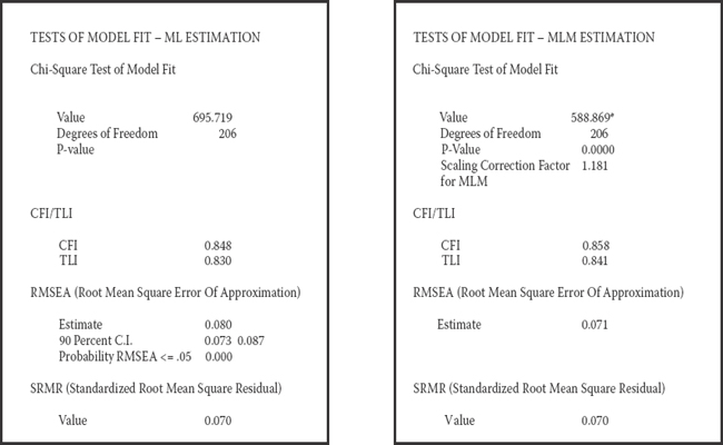
Figure 4.3. Mplus output files showing goodness-of-fit statistics based on ML estimation (on the left) and on MLM estimation (on the right).
In addition to the discrepancy in χ2 values, note also that the scaling factor made a difference to both the CFI and TLI values, which are very slightly higher for the MLM, than for the ML estimator; likewise, the RMSEA value is lower. Although Mplus reports a 90% confidence interval for the ML estimate, no interval accompanies the robust RMSEA value.
Given that estimation of the hypothesized model based on the robust MLM estimator yielded results that appropriately represented the moderate nonnormality of the data, all subsequent discussion related to results of this initial test of the model will be based on the MLM output. Accordingly, let's turn once again to tests of model fit presented in Figure 4.3, albeit with specific attention to results for the MLM model. Although both the Standardized Root Mean Square Residual (SRMR; 0.070) and RMSEA (0.071) values are barely within the scope of adequate model fit, those for the CFI (0.858) and TLI (0.841) are clearly indicative of an ill-fitting model. To assist us in pinpointing possible areas of misfit, we examine the MIs. Of course, as noted in Chapter 3, it is important to realize that once we have determined that the hypothesized model represents a poor fit to the data (i.e., the null hypothesis has been rejected) and subsequently embark upon post hoc model fitting to identify areas of misfit in the model, we cease to operate in a confirmatory mode of analysis. All model specification and estimation henceforth represent exploratory analyses. We turn now to the issue of misspecification with respect to our hypothesized model.
Model Misspecification
Recall from Chapter 3 that the targets of model modification are only those parameters specified as constrained either to zero or to some nonzero value, or as equal to some other estimated parameter. In this chapter, only parameters constrained to zero are of interest, with the primary focus being the factor loadings and observed variable residual covariances. As such, the zero factor loadings represent the loading of an item on a nontarget factor (i.e., a factor the item was not designed to measure). Zero values for the residual covariances, of course, simply represent the fact that none of the item residual variances are correlated with one another. In reviewing misspecification results for the factor loadings (listed under the BY statements), large MI values argue for the presence of factor cross-loadings (i.e., a loading on more than one factor), whereas large MIs appearing under the WITH statements represent the presence of residual covariances. Let's turn now to Table 4.1, where the MIs resulting from this initial test of the hypothesized model are reported.
Table 4.1 Mplus Output: Modification Indices (MIs) for Hypothesized Model
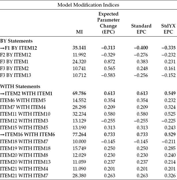
Although a review of the MIs presented here reveals a few very large values, two in particular stand apart from the rest (MI = 77.264; MI = 69.786). Both MIs signify residual covariances, with the larger of the two representing a residual covariance between Item 16 and Item 6, and the next largest representing a covariance between Item 1 and Item 2; both are flagged with boldface type. As you will recall from my extensive explanation of this topic in Chapter 3, the MI value of 77.264, for example, indicates that if this parameter were to be freely estimated, the overall χ2 statistic could decrease by approximately that amount.
Other important additional information is the expected parameter change (EPC) values, which, as you may recall from Chapter 3, represent the approximate value that a parameter is expected to attain should it be subsequently estimated. In the case of both residual covariances here, the EPC values can be considered to be extremely high (Items 16/6 = 0.733; Items 2/1 = 0.613) and argue strongly for their model specification.
These measurement residual covariances represent systematic rather than random measurement error in item responses, and they may derive from characteristics specific either to the items or to the respondents (Aish & Jöreskog, 1990). For example, if these parameters reflect item characteristics, they may represent a small omitted factor. If, on the other hand, they represent respondent characteristics, they may reflect bias such as yeasaying or naysaying, social desirability, and the like (Aish & Jöreskog, 1990). Another type of method effect that can trigger residual covariances is a high degree of overlap in item content. Such redundancy occurs when an item, although worded differently, essentially asks the same question. I believe the latter situation to be the case here. For example, Item 16 asks whether working with people directly puts too much stress on the respondent, whereas Item 6 asks whether working with people all day puts a real strain on him or her.3
Although a review of the MIs related to the factor loadings reveals five parameters representative of cross-loadings, I draw your attention to the one with the highest value (MI = 35.141). This parameter, which represents the cross-loading of Item 12 on the EE factor, stands apart from the other three possible cross-loading misspecifications. Such misspecification, for example, could mean that Item 12, in addition to measuring personal accomplishment, also measures emotional exhaustion; alternatively, it could indicate that, although Item 12 was postulated to load on the PA factor, it may load more appropriately on the EE factor.
Post Hoc Analyses
Provided with information related both to model fit and to possible areas of model misspecification, a researcher may wish to consider respecifying an originally hypothesized model. As emphasized in Chapter 3 and noted earlier in this chapter, should this be the case, it is critically important to be cognizant of both the exploratory nature of and the dangers associated with the process of post hoc model fitting. Having determined (a) inadequate fit of the hypothesized model to the sample data, and (b) at least two substantially misspecified parameters in the model (e.g., the two residual covariances were originally specified as zero), it seems both reasonable and logical that we now move into exploratory mode and attempt to modify this model in a sound and responsible manner. Thus, for didactic purposes in illustrating the various aspects of post hoc model fitting, we'll proceed to respecify the initially hypothesized model of MBI structure taking this information into account.
Model respecification that includes correlated residuals, as with other parameters, must be supported by a strong substantive and/or empirical rationale (Jöreskog, 1993), and I believe that this condition exists here. In light of (a) apparent item content overlap, (b) the replication of these same residual covariances in previous MBI research (e.g., Byrne, 1991, 1993), and (c) Bentler and Chou's (1987) admonition that forcing large error terms to be uncorrelated is rarely appropriate with real data, I consider respecification of this initial model to be justified. Testing of this respecified model (Model 2) now falls within the framework of post hoc analyses. We turn now to this modification process.
Testing the Validity of Model 2
Respecification of the hypothesized model of MBI structure involves the addition of freely estimated parameters to the model. However, because the estimation of MIs in Mplus is based on a univariate approach (cf. EQS and a multivariate approach), it is critical that we add only one parameter at a time to the model as the MI values can change substantially from one tested parameterization to another. (An excellent example of such fluctuation is evidenced in Chapter 6 of this volume.) Thus, in building Model 2, it seems most reasonable to proceed first in adding to the model the residual covariance having the largest MI. Recall from Table 4.1 that this parameter represents the residual covariance between Items 6 and 16 and, according to the EPC statistic, should result in a parameter estimated value of approximately 0.733. The Mplus input file for Model 2 is shown in Figure 4.4.
Input File 2
In reviewing this revised input file, note the newly specified parameter representing a residual covariance between Item 6 and Item 16. The only other change to the original input file is the title, which indicates that the model under study is Model 2.
Output File 2
Selected results pertinent to the testing of Model 2 are reported in Table 4.2. Included here are the key model goodness-of-fit statistics, as well as the estimated value of the specified residual covariance between Items 6 and 16.
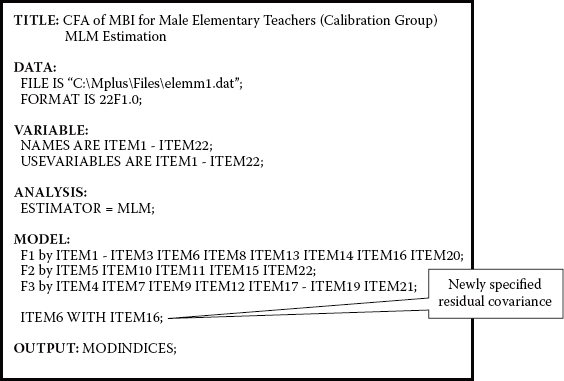
Figure 4.4. Mplus input file showing specification of the addition of a residual covariance between Items 6 and 16.
Turning first to the test of model fit, we find a substantial drop in the MLM χ2 from 588.869 to 507.188. It is important at this time for me to explain that when analyses are based on ML estimation, it has become customary to determine if the difference in fit between the two models is statistically significant. As such, the researcher examines the difference in χ2 (Δχ2) values between the two models. Doing so, however, presumes that the two models are nested.4 This difference between the models is itself χ2 distributed, with degrees of freedom equal to the difference in degrees of freedom (Δdf); it can thus be tested statistically, with a significant Δχ2 indicating substantial improvement in model fit. However, as the asterisk in Table 4.2 serves to remind us, when model comparisons are based on MLM estimation, it is inappropriate to calculate the difference between the two scaled χ2 values as they are not distributed as χ2. Although a formula is available for computing this differential (see the “Technical Appendices” on the Mplus website, http://www.statmodel.com; Bentler, 2005), there is no particular need to determine this information here. (A detailed example of how this differential value is computed will be illustrated in Chapter 6.) Suffice it to say that the inclusion of this one residual covariance to the model made a very influential difference to the model fit, which is also reflected in increased values for both the CFI (from 0.858 to 0.888) and TLI (from 0.841 to 0.874), albeit slightly lower values for the RMSEA (from 0.071 to 0.063) and SRMR (from 0.070 to 0.069).
Turning now to the model results in Table 4.2, we can see that the estimated value for the residual covariance is 0.733, exactly in tune with the predicted EPC value. With a standard error of 0.108, the z-value of this parameter is 6.772 (0.733/0.108), which is highly significant. Results from both the fit statistics and the estimated value for the residual covariance between Items 6 and 16 provide sound justification for the inclusion of this parameter in the model.
Table 4.2 Mplus Output for Model 2: Selected Goodness-of-Fit Statistics and Model Results
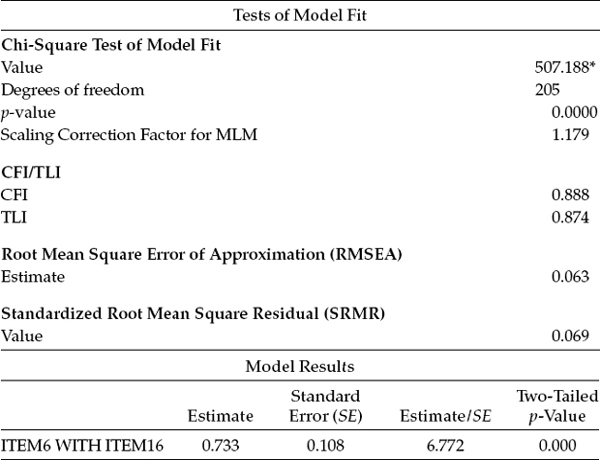
* The chi-square value for MLM, MLMV, MLR, ULSMV, WLSM, and WLSMV cannot be used for chi-square difference testing in the regular way. MLM, MLR, and WLSM chi-square difference testing is described on the Mplus website. MLMV, WLSMV, and ULSMV difference testing is done using the DIFFTEST option.
Let's now review the resulting MIs for Model 2, which are shown in Table 4.3. Here we observe that the residual covariance related to Items 1 and 2 remains a strongly misspecified parameter (MI = 66.418) in the model, with the EPC statistic suggesting that if this parameter were incorporated into the model, it would result in an estimated value of approximately 0.591, which, again, is exceptionally high. As with the residual covariance between Items 6 and 16, the one between Items 1 and 2 suggests redundancy due to content overlap. Item 1 asks if the respondent feels emotionally drained from his or her work, whereas Item 2 asks if the respondent feels used up at the end of the workday. Clearly, there appears to be an overlap of content between these two items.
Table 4.3 Mplus Output for Model 2: Modification Indices (MIs)
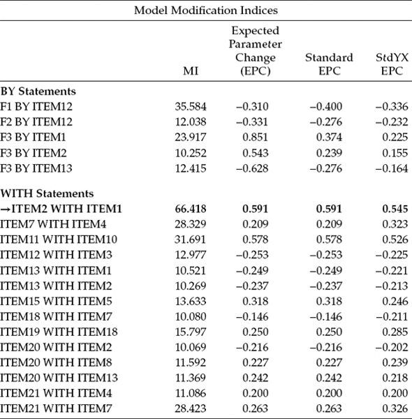
Given the strength of both the MI and EPC values for this residual covariance, together with the obvious overlap of item content, I recommend that this residual covariance parameter also be included in the respecified model, which we'll call Model 3. Let's move on, then, to the testing of this second respecified model.
Testing the Validity of Model 3
Specification of Model 3 is simply a matter of modifying the Model 2 input file (see Figure 4.4) such that it includes the additional WITH statement “ITEM 1 WITH ITEM 2.” Model fit statistics for this model, together with the resulting estimate for the residual covariance between Items 1 and 2, are shown in Table 4.4.
Table 4.4 Mplus Output for Model 3: Selected Goodness-of-Fit Statistics and Model Results
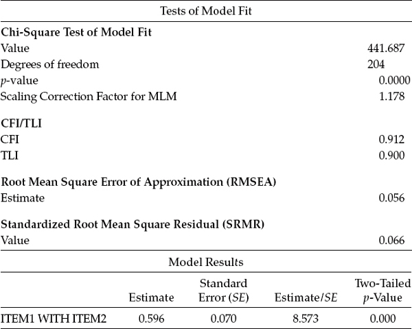
In reviewing goodness-of-fit statistics related to Model 3, we again observe a substantially large improvement in fit over that of Model 2 (MLM χ2[204] = 441.687 versus MLM χ2[205] = 507.188; CFI = 0.912 versus CFI = 0.888; TLI = 0.900 versus TLI = 0.874; and RMSEA = 0.056 versus RMSEA = 0.063).
Likewise, examination of the model results reveals the estimated value of the residual covariance between Items 1 and 2 to approximate its EPC value (see Table 4.4) and to be statistically significant (Estimate [Est]/ standard error [SE] = 8.573).
Turning to the MIs, presented in Table 4.5, we see that there is still at least one residual covariance with a fairly large MI (Item 11 with Item 10). Item 11 asks the teacher respondent if it is a concern that the job may be hardening him or her emotionally, whereas Item 10 asks if the teacher believes she or he has become more callous since taking the job.
In addition to this residual covariance, however, it is important to note results related to the misspecified factor loading (Item 12) noted earlier, as indicated by an MI value of 34.815, which is slightly higher than the MI value of 31.563 for the residual covariance. In the initially hypothesized model, this item was specified as loading on Factor 3 (Reduced Personal Accomplishment), yet the MI is telling us that it should additionally load on Factor 1 (Emotional Exhaustion). In trying to understand why this cross-loading might be occurring, let's take a look at the essence of the item content, which asks for a level of agreement or disagreement with the statement that the respondent feels very energetic. Although this item was deemed by Maslach and Jackson (1981, 1986) to measure a sense of personal accomplishment, it seems both evident and logical that it also taps one's feelings of emotional exhaustion. Ideally, items on a measuring instrument should clearly target only one of its underlying constructs (or factors).5 The question related to our analysis of the MBI, however, is whether or not to include this parameter in a third respecified model. Provided with some justification for the double-loading effect, together with evidence from the literature that this same cross-loading has been noted in other research, I consider it appropriate to respecify Model 4 with this parameter freely estimated.
Table 4.5 Mplus Output for Model 3: Modification Indices (MIs)
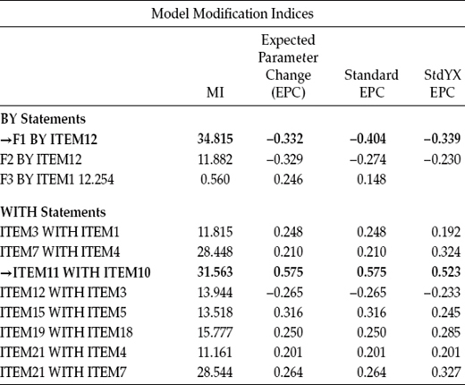
Given (a) the presence of these two clearly misspecified parameters (residual covariance between Items 10 and 11, and cross-loading of Item 12 on Factor 3), (b) the close proximity of their MI values, (c) the logical and substantively viable rationales for both respecifications, and (d) the need to keep a close eye on model parsimony, we face the question of how to proceed from here. Do we respecify the model to include the residual covariance, or do we respecify it to include a factor cross-loading? Presented with such results, it is prudent to also compare their EPC values. In this instance, we find that if the cross-loading were specified, the expected estimated value would be -0.332; in contrast, the expected estimate for the residual covariance would be 0.575. That the projected estimate for the residual covariance is the stronger of the two argues in favor of its selection over the cross-loading for inclusion in the model (see, e.g., Kaplan, 1989). Thus, with the residual covariance between Items 10 and 11 added to the (Model 3) input file, we now move on to test this newly respecified model, labeled here as Model 4. Goodness-of-fit results, together with the estimated value of this new parameter, are presented in Table 4.6.
In reviewing these results, we see that once again, there has been a substantial drop in the overall MLM χ2 (MLM χ2[203] = 413.639), as well as an increase in the CFI (0.922) and TLI (0.911), and a slight reduction in the RMSEA (0.053). Likewise, we observe that the estimated value of 0.519, although lower than the predicted value, is still highly significant as evidenced from its z-value of 5.030. Nonetheless, we are still presented with a model fit that is not completely adequate. Although still fully cognizant of the parsimony issue, yet aware of the two similarly sized MIs related to Model 3, I believe that we are fully justified in checking out the MIs on Model 4; these results are reported in Table 4.7.
Table 4.6 Mplus Output for Model 4: Selected Goodness-of-Fit Statistics and Model Results
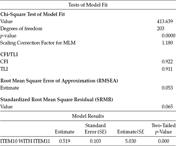
Table 4.7 Mplus Output for Model 4: Modification Indices
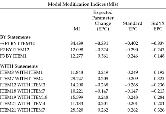
As expected, the cross-loading of Item 12 onto Factor 1 is still very strong, and its MI remains the highest value reported. Given that specification of this cross-loading can be logically and substantively supported, as noted earlier, we can proceed in testing a further model (Model 5) in which this parameter is included.
Although you will observe several remaining misspecified parameters, I consider it inappropriate to continue fitting the model beyond this point for at least three important reasons. First, given that we will have already added four parameters, despite the strong substantive justification for doing so, the issue of scientific parsimony must be taken into account. Second, of the nine remaining suggested misspecified parameters, seven represent residual covariances. Finally, in addition to having weaker MIs than the four previously acknowledged misspecified parameters, these remaining parameters are difficult to justify in terms of substantive meaningfulness. Model 5, then, represents our final model of MBI structure.
The Mplus input file for this final model is shown in Figure 4.5, and the resulting goodness-of-fit statistics are reported in Table 4.8. Turning first to the Mplus input file (Figure 4.5) and comparing it with the initial input file, I draw your attention to the four additionally specified parameters as derived from examination of the MIs related to post hoc analyses of the initially hypothesized model. As noted in the callouts, the first newly specified parameter represents the cross-loading of Item 12 on F1. The three additionally specified parameters appear below the factor loadings and represent residual covariances. Finally, the OUTPUT command has been revised to include only the STDYX standardized estimates.
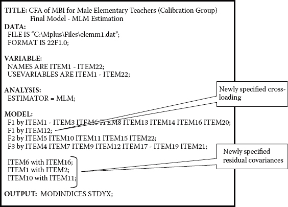
Figure 4.5. Mplus input file for a final model of MBI structure.
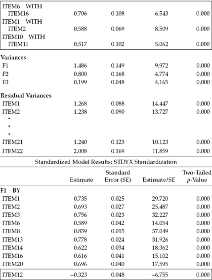
Let's turn now to the goodness-of-fit statistics presented in Table 4.8 and, in particular, to the CFI, TLI, RMSEA, and SRMR results. Both the CFI and TLI results represent a fairly well-fitting model, albeit one not quite reaching the recommended criterion of 0.95 (see Hu & Bentler, 1999). Nonetheless, both the RMSEA value of 0.048 and the SRMR value of 0.054 are indicative of good fit. Thus, these findings, in combination with the three important considerations noted earlier, stand in favor of allowing this fifth model to serve as the final model of MBI structure. Selected parameter estimates for this final model are reported in Table 4.9.
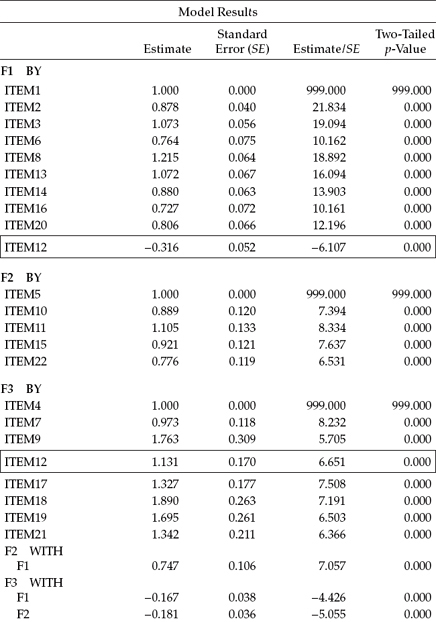
Both unstandardized and standardized parameter estimates are presented here as they appear in the Mplus output. In the interest of space, however, only the unstandardized estimates for the first and last four residual variances are included. All specified parameters were found to be statistically significant.
In reviewing these results, two sets of estimates are of primary import: (a) those related to the four post hoc–added parameters, and (b) the factor correlations. Turning first to the four additionally specified parameters, you will note that I have highlighted both the cross-loading and the residual covariances within rectangles with respect to both the unstandardized and standardized solutions. Let's examine the cross-loading of Item 12 on Factors 1 and 3 first. Recall that the originally intended loading of Item 12 was on Factor 3; the post hoc analyses, however, revealed a very strong misspecification indicating that this item should also load on Factor 1. As shown in Table 4.9 for the unstandardized estimates, both parameterizations were found to be highly significant. That the estimated loading on Factor 1 had a negative value is perfectly reasonable as the item states that the respondent feels very energetic, albeit Factor 1 represents the construct of Emotional Exhaustion. Turning to the standardized solution, it is not surprising to find that Item 12 has very similar and moderately high loadings on both factors (Factor 1 = -0.323; Factor 3 = 0.424). This finding attests to the fact that Item 12 is in definite need of modification such that it more appropriately loads cleanly on only one of these two factors.
Table 4.8 Mplus Output for Final Model: Selected Goodness-of-Fit Statistics
| Tests of Model Fit | |
| Chi-Square Test of Model Fit | |
| Value | 378.656 |
| Degrees of freedom | 202 |
| p-value | 0.0000 |
| Scaling Correction Factor for MLM | 1.179 |
| CFI/TLI | |
| CFI | 0.934 |
| TLI | 0.925 |
| Root Mean Square Error of Approximation (RMSEA) | |
| Root Mean Square Error of Approximation (RMSEA) | 0.048 |
| Standardized Root Mean Square Residual (SRMR) | |
| Value | 0.054 |
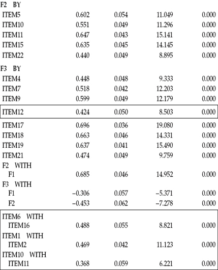
In reviewing the three residual covariances, we see that not only are they highly significant parameters in the model, but also they represent extremely high correlated residuals, ranging from 0.368 to 0.488. Such results are highly suggestive of excessively redundant item content.
Our second important focus concerned the latent factor correlations. Of critical import here is the extent to which these values are consistent with the theory. Based on previous construct validity research on the MBI, the correlational values of 0.685, -0.306, and -0.453 for Factor 1 (Emotional Exhaustion) with Factor 2 (Depersonalization), Factor 1 with Factor 3 (Personal Accomplishment), and Factor 2 with Factor 3, respectively, are strongly supported in the literature.
Table 4.9 Mplus Output for Final Model: Parameter Estimates
In closing out this chapter, albeit prior to the inclusion of the addendum, I wish to address the issue of post hoc model fitting, as, historically, one of the major concerns in this regard has been the potential for capitalization on chance factors in the respecification of alternate models. Indeed, there has been some attempt to address this issue. In 1999, Hancock introduced a Scheffé-type adjustment procedure that is now implemented in the EQS program (Bentler, 2005). However, this approach to controlling for Type I error is very conservative, leading Bentler (2005) to caution that, in practice, this criterion will likely be helpful only in situations where there are huge misspecifications in a model (χ2/df = or > 5.0).
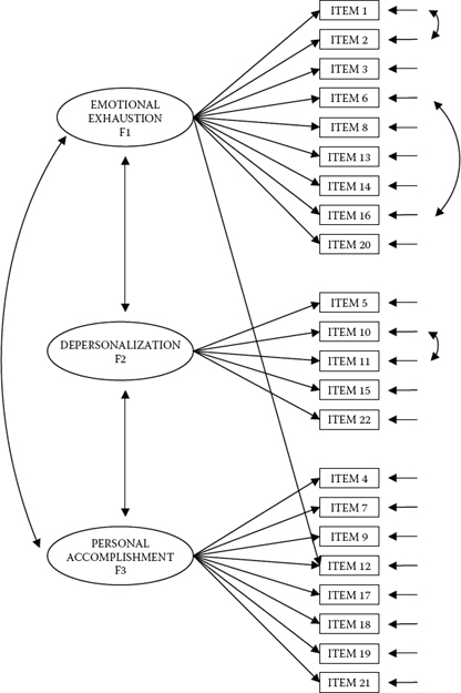
Figure 4.6. Final model of MBI structure.
Taking a different approach to the problem of Type I errors in post hoc model fitting, Green and colleagues (Green & Babyak, 1997; Green, Thompson, & Poirier, 2001) proposed a Bonferroni-type correction to the number of parameters added to a respecified model during post hoc analyses. Although a third approach to controlling for Type I errors was originally informally suggested by Chou and Bentler (1990), it was later regenerated and presented in a more formal manner by Green, Thompson, and Poirier (1999). This strategy is based on a two-step process in which parameters are first added to the model in the process of optimizing model fit, and then subsequently tested and deleted from the model if they cease to contribute importantly to model fit. Finally, a fourth approach to the problem of chance factors is to cross-validate the final model in a second independent new or split sample. Indeed, my own work with the MBI has provided me with the opportunity to test for the replication of the four misspecified parameters found in this chapter across split and independent samples. Results have revealed consistent problems with the seven MBI items cited in the present application across calibration and validation samples, as well as across elementary, intermediate, secondary, and postsecondary educators (see Byrne, 1991, 1993, 1994b); total replication of the residual covariances has been found across elementary and secondary teachers, as well as across gender (see Byrne 1994a). I address the issue of cross-validation more fully in Chapter 9.
In this chapter, we have tested for the validity of scores derived from the MBI for a sample of male elementary school teachers. Based on sound statistical and theoretical rationales, we can feel confident that the modified model of MBI structure, as determined through post hoc model-fitting procedures based on both the Modification Index results and determined substantive meaningfulness of the targeted misspecified parameters, most appropriately represents the data. A schematic summary of this final well-fitting model is presented in Figure 4.6.
Notes
| 1. | As was the case in Chapter 3, the first of each congeneric set of items was constrained to 1.00 by default by the program. |
| 2. | Mplus also provides for use of the MLMV estimator. Although the MLM and MLMV yield the same estimates (equivalent to ML) and standard errors (robust to nonnormality), their χ2 values differ and are corrected in both cases. Whereas the MLM χ2 is based on mean correction, the MLMV χ2 is based on mean and variance correction. As a consequence, one should expect p-values of the MLMV-corrected χ2 to be more accurate than for the MLM–corrected χ2, albeit at the expense of a greater number of computations. This computational difference between MLM and MLMV estimations is most apparent in the analysis of models that include a large number of variables. |
| 3. | Unfortunately, refusal of copyright permission by the MBI test publisher prevents me from presenting the actual item statements for your perusal. |
| 4. | As noted earlier in this book, nested models are hierarchically related to one another in the sense that their parameter sets are subsets of one another (i.e., particular parameters are freely estimated in one model but fixed to zero in a second model) (Bentler & Chou, 1987; Bollen, 1989). |
| 5. | Prior to specifying the cross-loading here, I would suggest loading the aberrant item onto the alternate factor in lieu of its originally targeted factor. However, in the case of Item 12, past experience has shown this item to present the same misspecification results regardless of which factor it is specified to load on. |
Addendum
The purpose of this addendum is to illustrate steps to follow in acquiring univariate skewness and kurtosis statistics pertinent to one's data using Mplus. As such, we now examine both the input file and output file results based on the present data. We turn first to the related input file, which is presented in Figure 4.7.
Of initial note with this input file is the ANALYSIS command, which states that TYPE = MIXTURE. The rationale behind this specification is related to the fact that, in order to obtain values of univariate skewness and kurtosis in Mplus, it is necessary to specify a mixture model. However, whereas the latent variables in mixture models are categorical (Brown, 2006), those in all models tested in this book are continuous.

Figure 4.7. Mplus input file for obtaining skewness and kurtosis values of observed variables.
Given that our model does not represent a mixture model and is pertinent to only one group (or class), the procedure here requires that two important specification statements be included in the input file: (a) CLASSES = c (1), as shown under the VARIABLE command; and (b) %OVERALL%, as shown on the first line of the MODEL command. The first statement (in the VARIABLE command) indicates that the model is of a regular non-mixture type pertinent to only one class. The second statement (in the MODEL command) indicates that the model describes the overall part of a specified nonmixture model. The remainder of the MODEL command, consistent with Figure 4.1, specifies that Factor 1 is measured by Items 1, 2, 3, 6, 8, 13, 14, 16, and 20; Factor 2 by Items 5, 10, 11, 15, and 22; and Factor 3 by Items 4, 7, 9, 12, 17, 18, 19, and 21. Finally, the OUTPUT command requests the TECH12 option, which yields information related to univariate skewness and kurtosis.
Let's now review the results of the TECH12 output, which are presented in Figure 4.8. As noted earlier, given that kurtosis remains the primary concern in analyses of covariance structures (the present case), we focus only on these values. As such, a review of these kurtosis values reveals that, in general, most are quite acceptable as they deviate minimally from zero. Nonetheless, there are four observed variables that may be of concern: Items 4, 7, 15, and 17, each of which is shown as circled in Figure 4.8.
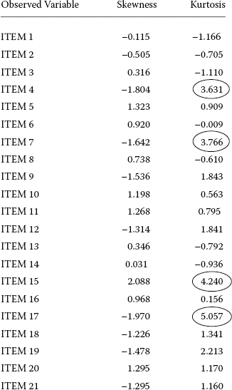
Figure 4.8. Mplus output results for univariate skewness and kurtosis values.
Although the four aberrant items noted here are clearly not excessively kurtotic, they may nonetheless be sufficiently nonnormal to make interpretations based on the ML χ2 statistic, as well as the CFI, TLI, and RMSEA indices, problematic. Thus, it is always best to err on the side of caution by taking this information into account, which is exactly what we did in our analyses of the MBI data in this chapter.