
chapter 5
Testing the Factorial
Validity of Scores From a
Measuring Instrument
Second-Order Confirmatory
Factor Analysis Model
The application to be illustrated in this chapter differs from those of the previous chapters in two ways. First, it focuses on a confirmatory factor analysis (CFA) model that comprises a second-order factor structure. Second, whereas analyses in Chapters 3 and 4 were based on continuous data, analyses in the present application are based on categorical data. As such, the ordinality of the item data is taken into account. Specifically, in this chapter, we test hypothesized factorial structure related to the Chinese version (Chinese Behavioral Sciences Society, 2000) of the Beck Depression Inventory-II (BDI-II; Beck, Steer, & Brown, 1996) as it bears on a community sample of adolescents. The example is taken from a study by Byrne, Stewart, and Lee (2004). Although this particular study was based on an updated version of the original BDI (Beck, Ward, Mendelson, Mock, & Erbaugh, 1961), it nonetheless follows from a series of studies that have tested for the validity of second-order BDI factorial structure for high school adolescents in Canada (Byrne & Baron, 1993, 1994; Byrne, Baron, & Campbell, 1993, 1994), Sweden (Byrne, Baron, Larsson, & Melin, 1995, 1996), and Bulgaria (Byrne, Baron, & Balev, 1996, 1998). The purposes of the original Byrne et al. (2004) study were to test for construct validity of the structure of the Chinese version of the BDI-II (C-BDI-II) based on three independent groups of students drawn from 11 Hong Kong high schools. In this example, we focus only on the Group 2 data (N = 486), which served as the calibration sample in testing for the factorial validity of the C-BDI-II. (For further details regarding the sample, analyses, and results, readers are referred to the original article.)
The C-BDI-II is a 21-item scale that measures symptoms related to cognitive, behavioral, affective, and somatic components of depression. Specific to the Byrne et al. (2004) study, only 20 of the 21 C-BDI-II items were used in tapping depressive symptoms for high school adolescents. Item 21, designed to assess changes in sexual interest, was considered to be objectionable by several school principals, and the item was subsequently deleted from the inventory. For each item, respondents are presented with four statements rated from 0 to 3 in terms of intensity, and they are asked to select the one that most accurately describes their own feelings; higher scores represent a more severe level of reported depression. As noted in Chapter 4, the CFA of a measuring instrument is most appropriately conducted with fully developed assessment measures that have demonstrated satisfactory factorial validity. Justification for CFA procedures in the present instance is based on evidence provided by Tanaka and Huba (1984), and replicated studies by Byrne and associates (Byrne & Baron, 1993, 1994; Byrne, Baron, & Campbell, 1993, 1994; Byrne, Baron, Larsson, & Melin, 1995, 1996; Byrne, Baron, & Balev, 1996, 1998), that BDI score data are most adequately represented by a hierarchical factorial structure. That is to say, the first-order factors are explained by some higher order structure that, in the case of the C-BDI-II, is a single second-order factor of general depression.
Let's turn now to a description of the postulated structure of the C-BDI-II.
The Hypothesized Model
The CFA model tested in the present application hypothesizes a priori that (a) responses to the C-BDI-II can be explained by three first-order factors (Negative Attitude, Performance Difficulty, and Somatic Elements) and one second-order factor (General Depression); (b) each item has a nonzero loading on the first-order factor it was designed to measure, and zero loadings on the other two first-order factors; (c) residuals associated with each item are uncorrelated; and (d) covariation among the three first-order factors is explained fully by their regression on the second-order factor. A diagrammatic representation of this model is presented in Figure 5.1.
One additionally important point I need to make concerning this model is that, in contrast to the CFA models examined in Chapters 3 and 4, the first factor loading of each congeneric set of indicator variables is not fixed to 1.0 for purposes of model identification and latent variable scaling. Rather, these fixed values are specified for the factor loadings associated with CBDI2_3 for Factor 1, CBDI2_12 for Factor 2, and CBDI2_16 for Factor 3, as indicated in Figure 5.1.1
Analysis of Categorical Data
Thus far in the book, analyses have been based on maximum likelihood (ML) estimation (Chapter 3) and robust ML (MLM) estimation (Chapter 4).
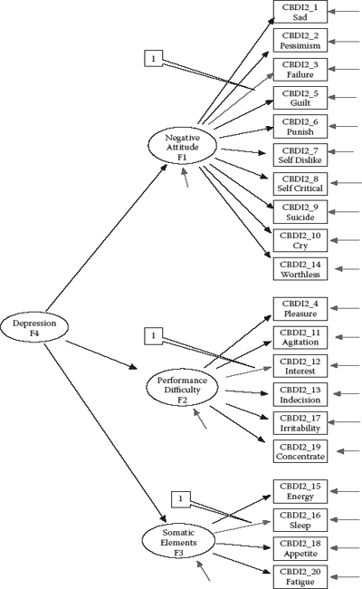
Figure 5.1. Hypothesized second-order model of factorial structure for the Chinese version of the Beck Depression Inventory II.
An important assumption underlying both of these estimation procedures is that the scale of the observed variables is continuous. Although, admittedly, the data analyzed in Chapter 4 involved Likert-scaled items that, technically speaking, represented categorical data, they were treated as if they were continuous on the basis of the relatively large number of scale points upon which the instrument items were based. (This issue is addressed shortly.) In contrast, the C-BDI-II data used in the present application comprise items having four scale points, and it is appropriate for analyses to take this categorical nature of the data into account.
For many years, researchers have tended to treat categorical data as if they were continuous. This trend applies to traditional statistical techniques (e.g., ANOVA and MANOVA) as well as to structural equation modeling (SEM) analyses. The primary reason this practice occurred with respect to SEM analyses, in particular, was because there were no well-developed strategies for addressing the categorical nature of the data. Despite the seminal work of Muthén (1978, 1983, 1984, 1993) in advancing the need to address the categorical nature of data with appropriate analytic methods, accompanied by his development of LISCOMP (Muthén, 1987), a computer program (and forerunner of Mplus) capable of meeting this challenge, it has really been only in the last decade or so that SEM researchers have begun to act upon these earlier caveats. Clearly, methodological advancements both in the development of estimators capable of analyzing categorical data and in their incorporation into the major SEM computer software packages have played a major role not only in heightening researchers’ awareness to the importance of addressing the categorical nature of data but also in enabling them to apply these appropriate analytic procedures.
This changing trend among SEM researchers notwithstanding, it would be reasonable for you to query (a) how serious it is to treat categorical data as if they are continuous, and (b) if there are instances where it makes little difference whether the data are treated as categorical or as continuous. Thus, before discussing the basic framework underlying the analysis of categorical variables, I believe a brief review of the literature that has addressed these issues may be of substantial help in providing you with a broader perspective of the two analytic strategies. We turn first to the case where categorical variables are treated as if they are continuous variables, and then to their treatment as categorical variables.
Categorical Variables Analyzed as Continuous Variables
From a review of Monte Carlo studies that have addressed this issue (see, e.g., Babakus, Ferguson, & Jöreskog, 1987; Boomsma, 1982; Muthén & Kaplan, 1985), West, Finch, and Curran (1995) reported several important findings. First, Pearson correlation coefficients appear to be higher when computed between two continuous variables than when computed between the same two variables restructured with an ordered categorical scale. However, the greatest attenuation occurs with variables having less than five categories and those exhibiting a high degree of skewness, the latter condition being made worse by variables that are skewed in opposite directions (i.e., one variable positively skewed, and the other negatively skewed; see Bollen & Barb, 1981). Second, when categorical variables approximate a normal distribution:
- The number of categories has little effect on the χ2 likelihood ratio test of model fit. Nonetheless, increasing skewness, and particularly differential skewness (variables skewed in opposite directions), leads to increasingly inflated χ2 values.
- Factor loadings and factor correlations are only modestly underestimated. However, underestimation becomes more critical when there are fewer than three categories, skewness is greater than 1.0, and differential skewness occurs across variables.
- Residual variance estimates, more so than other parameters, appear to be most sensitive to the categorical and skewness issues noted in Item 2.
- Standard error estimates for all parameters tend to be too low, with this result being more so when the distributions are highly and differentially skewed (see also Finch, West, & MacKinnon, 1997).
In summary, the literature to date would appear to support the notion that when the number of categories is large and the data approximate a normal distribution, failure to address the ordinality of the data is likely negligible (Atkinson, 1988; Babakus et al., 1987; Muthén & Kaplan, 1985). Indeed, Bentler and Chou (1987) argued that, given normally distributed categorical variables, “continuous methods can be used with little worry when a variable has four or more categories” (p. 88). More recent findings support these earlier contentions and have further shown that (a) the χ2 statistic is influenced most by the two-category response format and becomes less so as the number of categories increases (Green, Akey, Fleming, Hershberger, & Marquis, 1997), (b) attenuation of parameter estimates may be heightened in the presence of floor and ceiling effects (Brown, 2006), and (c) there is a risk of yielding “pseudo-factors” that may be artifacts of item difficulty and extremeness (Brown, 2006).
Categorical Variables Analyzed as Categorical Variables
The Theory
In addressing the categorical nature of observed variables, the researcher automatically assumes that each has an underlying continuous scale. As such, the categories can be regarded as only crude measurements of an unobserved variable that, in truth, has a continuous scale (Jöreskog & Sörbom, 1993), with each pair of thresholds (or initial scale points) representing a portion of the continuous scale. The crudeness of these measurements arises from the splitting of the continuous scale of the construct into a fixed number of ordered categories (DiStefano, 2002). Indeed, this categorization process led O'Brien (1985) to argue that the analysis of Likert-scaled data actually contributes to two types of error: (a) categorization error resulting from the splitting of the continuous scale into the categorical scale, and (b) transformation error resulting from categories of unequal widths.
For purposes of illustration, let's consider the measuring instrument under study in this current chapter, in which each item is structured on a 4-point scale, thereby representing polytomous categorical variables. I draw from the work of Jöreskog and Sörbom (1993) in describing the decomposition of these categorical variables, albeit I replace the original use of the letter z with the letter y for consistency with the work of Muthén (1983, 1984) and Muthén and Muthén (2007–2010). Accordingly, let y represent the categorical variable (i.e., the item, the dependent indicator variable in the CFA model), and y* the unobserved and underlying continuous variable. The threshold values can then be conceptualized as follows:
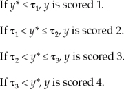
where τ represents tau (a vector containing threshold information), and τ1 < τ2 < τ3 represents threshold values for y*. The number of thresholds will always be one less than the number of categories.2
In testing SEM models with categorical data, analyses are no longer based on the sample variance–covariance matrix (S) as is the case for continuous data. Rather, they must be based on the correct correlation matrix. Where the correlated variables are both of an ordinal scale, the resulting matrix will comprise polychoric correlations; where one variable is of an ordinal scale, and the other of a continuous scale, the resulting matrix will comprise polyserial correlations. If two variables are dichotomous, this special case of a polychoric correlation is called a tetrachoric correlation. If a polyserial correlation involves a dichotomous rather than a more general ordinal variable, the polyserial correlation is also called a biserial correlation.
Underlying Assumptions
Applications involving the use of categorical data are based on three critically important assumptions: (a) Underlying each categorical observed variable is an unobserved latent counterpart, the scale of which is both continuous and normally distributed; (b) sample size is sufficiently large to enable reliable estimation of the related correlation matrix; and (c) the number of observed variables is kept to a minimum. However, Bentler (2005) noted that it is this very set of assumptions that essentially epitomizes the primary weakness in this methodology. Let's now take a brief look at why this should be so.
That each categorical variable has an underlying continuous and normally distributed scale is undoubtedly a difficult criterion to meet and, in fact, may be totally unrealistic. For example, in the present chapter, we examine scores tapping aspects of depression for nonclinical adolescents. Clearly, we would expect such item scores for normal adolescents to be low, thereby reflecting no incidence of depressive symptoms. As a consequence, we can expect to find evidence of kurtosis, and possibly skewness, related to these variables, with this pattern being reflected in their presumed underlying continuous distribution. Consequently, in the event that the model under test is deemed to be less than adequate, it may well be that the normality assumption is unreasonable in this instance.
The rationale underlying the latter two assumptions stems from the fact that, in working with categorical variables, analyses must proceed from a frequency table comprising the number of thresholds, multiplied by the number of observed variables, to estimation of the correlation matrix. The problem here lies with the occurrence of cells having zero or near-zero cases, which can subsequently lead to estimation difficulties (Bentler, 2005). This problem can arise because (a) sample size is small relative to the number of response categories (i.e., specific category scores across all categorical variables), (b) the number of variables is excessively large, and/ or (c) the number of thresholds is large. Taken in combination, then, the larger the number of observed variables and/or number of thresholds for these variables, and the smaller the sample size, the greater the chance of having cells comprising zero to near-zero cases.
General Analytic Strategies
Until approximately a decade or so ago, two primary approaches to the analysis of categorical data (Jöreskog, 1990, 1994; Muthén, 1984) have dominated this area of research. Both methodologies use standard estimates of polychoric and polyserial correlations, followed by modified implementation of the asymptotic distribution-free (ADF) estimator originally proposed by Browne (1982, 1984a); it is also known as the weighted least squares (WLS) estimator and is more commonly referred to as such today. Unfortunately, the positive aspects of these original categorical variable methodologies have been offset by the ultrarestrictive assumptions noted earlier that, for most practitioners, are both impractical and difficult to meet. Of particular note is the requirement of an exceptionally large sample size in order to yield stable estimates. For example, Jöreskog and Sörbom (1996) proposed, as a minimal sample size, (k + 1) (k + 2) / 2, where k represents the number of indicators in the model to be tested; alternatively, Raykov and Marcoulides (2000) recommended that sample size be greater than 10 times the number of estimated model parameters. (For an excellent recapitulation of this issue, readers are referred to Flora & Curran, 2004.)
Although attempts to resolve these difficulties over the past few years have resulted in the development of several different approaches to the modeling and testing of categorical data (see, e.g., Bentler, 2005; Coenders, Satorra, & Saris, 1997; Moustaki, 2001; Muthén & Muthén, 2007–2010), there appear to be only three primary estimators: unweighted least squares (ULS), WLS, and diagonally weighted least squares (DWLS). Corrections to the estimated means and/or means and variances based on only ULS and DWLS estimation yield their related robust versions as follows: correction to means and variances of ULS estimates (ULSMV), correction to means of DWLS estimates (WLSM), and correction to means and variances of DWLS estimates (WLSMV).3 (Admittedly, the interweaving of the WLS and DWLS labeling is unnecessarily confusing.) Of these, Brown (2006) contended that the WLSMV estimator performs best in the CFA modeling of categorical data.
The WLSMV estimator was developed by Muthén, du Toit, and Spisic (1997) based on earlier robustness research reported by Satorra and Bentler (1986, 1988, 1990) and designed specifically for use with small and moderate sample sizes (at least in comparison with those needed for use with the WLS estimator). The parameter estimates derive from use of a diagonal weight matrix (W), robust standard errors, and a robust mean- and variance-adjusted χ2 statistic (Brown, 2006). Thus, the robust goodness-of-fit test of model fit can be considered analogous to the Satorra-Bentler-scaled χ2 statistic that was the basis of our work in Chapter 4. Subsequent simulation research related to the WLSMV estimator has shown it to yield accurate test statistics, parameter estimates, and standard errors under both normal and nonnormal latent response distributions4 across sample sizes ranging from 100 to 1,000, as well as across four different CFA models (one-factor models with 5 and 10 indicators, and two-factor models with 5 and 10 indicators; see Flora & Curran, 2004). More recently, Beauducel and Herzberg (2006) also reported satisfactory results for the WLSMV estimator, albeit findings of superior model fit and more precise factor loadings when the number of categories is low (e.g., two or three categories, compared with four, five, or six). Mplus currently offers seven estimators (see Muthén & Muthén, 2007–2010) for use with data comprising at least one binary or ordered categorical indicator variable; the WLSMV estimator is default. As this book goes to press, the WLSMV estimator is available only in Mplus.
Now that you have some idea of the issues involved in the analysis of categorical variables, let's move on to our task at hand, which is to test a second-order CFA model based on the C-BDI-II data described at the beginning of this chapter.
Mplus Input File Specification and Output File Results
Input File
Four features of the present application differ from the previous two and, thus, are of interest here with respect to composition of the Mplus input file: (a) The CFA model is hierarchically structured, (b) the data upon which the analysis is based are ordinally scaled, (c) the factor-loading paths fixed to 1.0 for purposes of identification and scaling differ from the Mplus defaulted paths, and (d) one equality constraint has been specified with respect to the higher order structure. Presented here are two versions of this input file. The input file shown first in Figure 5.2 (Input file a), with the exception of the alternative fixed factor loadings, represents what would be considered the usual default version of the model shown in Figure 5.1. Given that WLSMV is the default estimator for analyses of categorical variables in Mplus, it need not be specified. In addition, the first factorloading path for each congeneric set of parameters would automatically be constrained to 1.0 and, thus, requires no specification. Finally, no equality constraints would be placed at the second-order level of the model.
The input file presented in Figure 5.3 (Input file b) represents the alternative specification to be used in our analyses here. For clarification, I have included the ANALYSIS command and specified the WLSMV estimator, although this is not necessary (as noted above). Turning next to the MODEL command, we focus first on the first-order factors, the specifications for which are shown in the first three lines of this input information. Of import here is the inclusion of asterisks assigned to variables CBDI2_1, CBDI2_4, and CBDI2_15. A review of the CFA model in Figure 5.1 reveals these three parameters (in contrast to the usual defaulted constraints of 1.0) to be freely estimated. Alternatively, the parameters CBDI2_3, CBDI2_12, and CBDI2_16 are constrained to a value of 1.0 and hence now serve as the reference indicator variables in the model. Accordingly, in Figure 5.3, you will observe that each of these latter parameters is specified as the appropriately fixed parameter through the addition of (e.g., CBDI2_3@1).
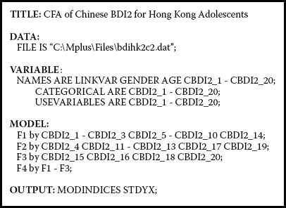
Figure 5.2. Mplus input file based on usual program defaults.
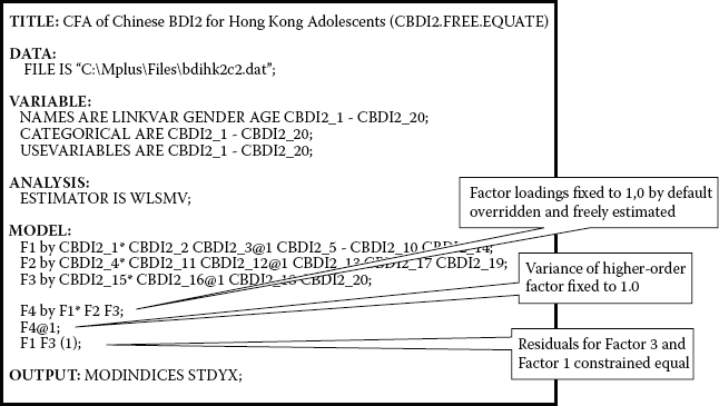
Figure 5.3. Mplus input file with alternative specification and no program defaults.
Let's turn now to the last three lines of the MODEL input, which contains specifications related to the second-order factor structure. Within this set of specifications, the first two lines again refer to a modification of the reference indicator variables, albeit this time with respect to the higher order factor loadings. That is, by default, Mplus would automatically constrain the first second-order factor-loading path (F4 → F1) to 1.0. However, because in specifying a higher order model, researchers are particularly interested in the estimation of the higher order factor loadings, there is some preference for freely estimating each of these parameters. An important corollary in SEM states that either a regression path or a variance can be estimated, but not both. The underlying rationale of this corollary is linked to the issue of model identification. Thus, if we wish to freely estimate all second-order factor loadings, we will need to constrain the variance of the second-order factor (F4, Depression) to a value of 1.0; otherwise, it would automatically be freely estimated by default. Because it can be instructive to see what happens if this corollary is not adhered to, I executed this file without fixing the F4 variance to 1.00. Accordingly, shown in Figure 5.4 is the error message generated by Mplus resulting from the estimation of this model wherein all second-order factor loadings were freely estimated, as well as the variance of Factor 4.
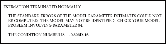
Figure 5.4. Mplus error message regarding higher order factor specifications.
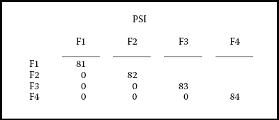
Figure 5.5. Mplus TECH1 output for factor covariance matrix (PSI).
Note in Figure 5.4 that Mplus identifies Parameter 84 as the source of the problem. In checking the related output file, as shown in Figure 5.5, we see that this parameter is none other than the higher order Factor 4, which needs to be constrained to 1.0 in order that the model is identified. In addressing this identification corollary, then, note on the second line of the higher order factor specification (see Figure 5.3) that Factor 4 has been assigned a fixed value of 1.0 (F4@1;).
The final specification of note lies on line 3 of this higher order set of specifications, where you will see the “F1 F3 (1);” statement. This specification indicates that the residual variances associated with Factors 1 and 3 are to be constrained equal. Technically speaking, the estimate for F3 will be constrained equal to the estimate for F1. The parenthesized value of 1 indicates that only one constraint has been specified, and it pertains to both F1 and F3. In Mplus, each specified constraint must appear on a separate line. Thus, for example, if the higher order model were to comprise six factors (in lieu of the present three), and if we wanted to equate two additional residual variances (say, F5 and F6, also with F1 and F3), the related constraint specification would appear on a separate line but still be accompanied by a bracketted value of 1 (“F1 F3 F5 F6 [1]”). If, on the other hand, we were to equate the estimate of F6 to that of F5, then this would represent an entirely different constraint and, thus, would be accompanied by the number 2 in brackets (“F5 F6 [2]”).
What is the rationale for such specification? Recall that in Chapters 2 and 3, I emphasized the importance of computing the degrees of freedom associated with hypothesized models in order to ascertain their status with respect to statistical identification. I further noted that, with hierarchical models, it is additionally critical to check the identification status of the higher order portion of the model. For example, in the case of a second-order factor model, the first-order factors replace the observed variables in serving as the data upon which second-order model identification is based. In the present case, given the specification of only three first-order factors, the higher order structure will be just-identified unless a constraint is placed on at least one parameter in this upper level of the model (see, e.g., Bentler, 2005; Rindskopf & Rose, 1988). More specifically, with three first-order factors, we have six ([4 ×; 3] / 2) pieces of information; the number of estimable parameters is also six (three factor loadings and three residual variances), thereby resulting in a just-identified model. Although acceptable in general terms, should we wish to resolve this condition of just identification, equality constraints can be placed on particular parameters known to yield estimates that are approximately equal. From earlier work in validating the C-BDI-II (Byrne et al., 2004), an initial test of the hypothesized model shown in Figure 5.1 revealed the estimates for the residual variances associated with F1 and F3 to be very close. Accordingly, these two parameters were constrained equal, thereby providing one degree of freedom at the higher order level of the model.
Output File
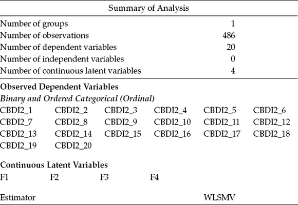
Table 5.1 presents the summary information appearing first in the Mplus output file. Here we see that the sample size is 486 and the number of dependent variables is 20, independent variables 0, and continuous latent variables 4. The dependent variables, as usual, represent the 20 observed indicator variables (in this case, the C-BDI-II item scores), whereas the latent variables represent the three first-order and one second-order factors. Finally, the analyses are based on the WLSMV estimator.
Table 5.1 Mplus Output for Hypothesized Model: Selected Summary Information
Presented next in Table 5.2 are the proportions of sample respondents who endorsed each of the four categories. For one example of how to interpret these results, let's examine the reported numbers as they relate to Item 1 (CBDI2_1). This item elicits a response to the statement “I feel sad,” which resulted in 51% (0.508) of the sample indicating the absence of sad feelings. A review of this proportion information for all 20 items reveals that for 16 out of 20 items, most respondents opted for Category 1, thereby reflecting no evidence of depressive symptoms. In other words, proportion results pertinent to Category 1 exceeded those for Categories 2 through 4 for 16 out of the 20 C-BDI-II items.5 As such, it is apparent that these data reflect a leptokurtic pattern and are thus nonnormally distributed. However, given that the data represent a community sample of high school adolescents and, thus, no presence of depressive symptoms is expected, this finding is certainly not unexpected. Indeed, it actually represents the usual finding when the C-BDI-II as well as the BDI-I are used with normal adolescents.
Let's turn next to Table 5.3, in which the goodness-of-fit statistics are reported. The WLSMV robust χ2(82) of 200.504 represents a scaled (i.e., corrected) version of the usual chi-square statistic for which both the categorical and nonnormal natures of the data have been taken into account.
Table 5.2 Mplus Output for Hypothesized Model: Summary of Categorical Proportions
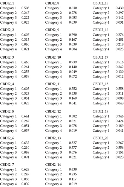
Table 5.3 Mplus Output for Hypothesized Model: Selected Goodness-of-Fit Statistics
| Tests of Model Fit | |
| Chi-Square Test of Model Fit | |
| Value | 200.504* |
| Degrees of freedom | 82** |
| p-value | 0.0000 |
| CFI/TLI | |
| CFI | 0.958 |
| TLI | 0.987 |
| Number of free parameters | 82 |
| Root Mean Square Error of Approximation (RMSEA) | |
| Estimate | 0.055 |
| Weighted Root Mean Square Residual (WRMR) | |
| Value | 0.947 |
* The chi-square value for MLM, MLMV, MLR, ULSMV, WLSM, and WLSMV cannot be used for chi-square difference tests. MLM, MLR, and WLSM chi-square difference testing is described in the Mplus “Technical Appendices” at the Mplus website, http://www.statmodel. com. See “chi-square difference testing” in the index of the Mplus User's Guide (Muthén & Muthén, 2007–2010).
**The degrees of freedom for MLMV, ULSMV, and WLSMV are estimated according to a formula given in the Mplus “Technical Appendices” at http://www.statmodel.com. See “degrees of freedom” in the index of the Mplus User's Guide (Muthén & Muthén, 2007–2010).
Accompanying this information are two asterisked notations. The first of these advises that, consistent with the MLM estimator (as noted in Chapter 4), no direct chi-square difference tests are permitted involving the WLSMV estimator, as this between-model value is not distributed as chi-square. Nonetheless, these tests are made possible via additional model testing, which is described and exemplified in Muthén and Muthén (2007–2010) as well as on the Mplus website (http://www.statmodel.com), and will be detailed in a walkthrough of this procedure relevant to the MLM estimator in Chapter 6. The second notation serves as a caveat that when the WLSMV estimator is used, calculation of degrees of freedom necessarily differs from the usual CFA procedure used with normally distributed continuous data as outlined earlier in this book. Interested readers can find details related to this computation from the Mplus website as noted in the output file.
A review of the remaining model fit statistics (CFI = 0.958; TLI = .987; RMSEA = 0.055) reveals the hypothesized model to exhibit a good fit to the data. Finally, given that the Weighted Root Mean Square Residual (WRMR) has been found to perform better than the Standardized Root Mean Square Residual (SRMR) with categorical data (Yu, 2002), only the WRMR value of 0.947 is repeated in the output. Indeed, Yu (2002) determined that a cutoff criterion of 0.95 can be regarded as indicative of good model fit with continuous as well as categorical data. As this book goes to press, the WLSMV estimator is still considered to be an experimental statistic (Mplus Product Support, April 23, 2010) and, thus, awaits further testing of its properties.
We turn next to the unstandardized parameter estimates, which are presented in Table 5.4. Note first that items CBDI2_3, CBDI2_12, and CBDI2_16 each has a value of 1.00 as they were the reference variables assigned to each congeneric set of factor loadings for Factors 1, 2, and 3, respectively. A review of both the first-order and second-order factor loadings reveals all to be statistically significant.
Table 5.4 Mplus Output for Hypothesized Model: Parameter Estimates
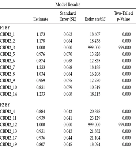
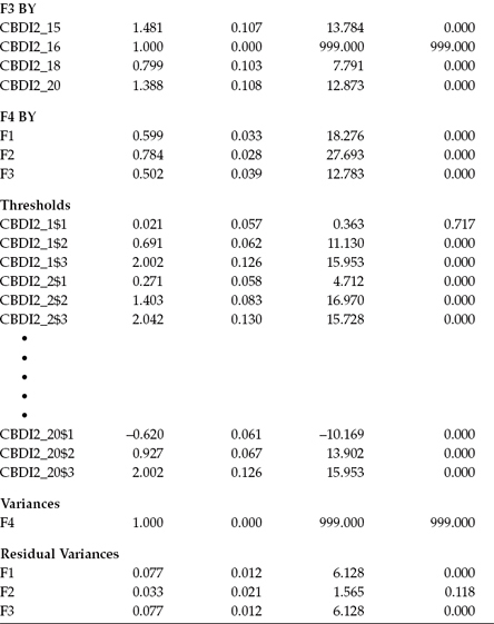
Appearing next in Table 5.4 are the thresholds specific to each C-BDI-II item. When observed indicator variables represent categorical item content, as noted earlier, there will be as many thresholds as there are categories less one. Thus, for each of the 20 items, we can expect to see three thresholds. In Mplus, these parameters are denoted by the assignment of a dollar sign ($) following the variable name. For example, the three thresholds for the first item, CBDI2_1, are CBDI2_1$1, CBDI2_1$2, and CBDI2_1$3. Due to constraints of space, only a subset of item threshold parameters is presented here.
The final two sets of parameters appearing here are (a) the variance for the higher order factor (Factor 4), which you will recall was fixed to 1.00; and (b) the residual variances associated with each of the first-order factor loadings. Recall that because these factors are themselves dependent latent variables in this CFA model (i.e., they have a single-headed arrow pointing at them) and therefore cannot have their variances estimated, the variances of their residuals are computed instead; their estimation is default in Mplus. Recall also that we constrained the estimated residual variance for Factor 3 to be equal to that for Factor 1. Thus, these two parameters have the same value (0.077), which is statistically significant (Estimate [Est]/standard error [SE] = 6.128). In contrast, the residual variance for Factor 2 is shown not to be significant (Est/SE = 1.565).
Notably missing in this output are residual variances for the observed categorical variables. Recall, however, that when SEM models involve categorical rather than continuous variables, analyses must be based on the appropriate sample correlation matrix (S),6 rather than on the sample covariance matrix. Because this correlation matrix represents the underlying continuous variable y*, the residual variances of categorical variables are not identified and therefore not estimated (Brown, 2006).
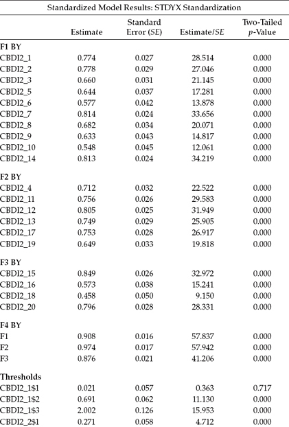
Given that the estimates in Tables 5.5 and 5.6 are linked statistically and, as such, bear importantly on their combined interpretation, I have chosen to present them as a pair. Table 5.5 presents the standardized estimates for each of the parameters listed in Table 5.4, whereas Table 5.6 reports the reliability estimates for each of the categorical variables (i.e., the items), in addition to the three first-order latent factors.
In the analysis of CFA models in which the observed variables are categorical (likewise for the measurement portion of full SEM path analytic models), the y* variances of these variables are standardized to 1.0. Thus, the parameter estimates should be interpreted accordingly (Brown, 2006). This caveat signifies that we should focus on the standardized, rather than on the unstandardized, estimates in our interpretation of the findings. For example, whereas factor-loading estimates for continuous variables are interpreted as the proportion of variance in the observed variables explained by the underlying factor, interpretation of factor-loading estimates for categorical variables is based on the squared standardized factor loadings. To see how this plays out, let's look at the standardized loading for CBDI2_1 (see Table 5.5), which is 0.774. Squaring this loading yields a value of 0.599, thereby representing the R2 estimate reported in Table 5.6 for the same variable (CBDI2_1). We interpret this value as representing the proportion of the variance in the underlying continuous and latent aspect ( y*) of CBDI2_1 that can be explained by Factor 1 of the hypothesized model. In other words, results for the first CBDI2 item (CBDI2_1) suggest that 60% of its variance (as represented by the latent continuous aspect of this categorical item) can be explained by the construct of Negative Attitude to which it is linked.
Table 5.5 Mplus Output for Hypothesized Model: Standardized Parameter Estimates
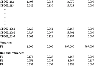
Likewise, residual variances express the proportion of y* variances that are not explained by the associated latent factor (Brown, 2006). Accordingly, keeping our focus on CBDI2_1, if we subtract the squared standardized loading (0.599) from 1.00, we obtain a value of 0.401, which you will note is reported as the residual variance for CBDI2_1 in Table 5.6.
Table 5.6 Mplus Output for Hypothesized Model: Reliability Estimates and Modification Indices
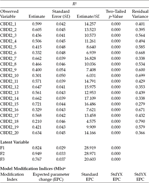
a Modification indices for direct effects of observed dependent variables regressed on covariates and residual covariances among observed dependent variables may not be included. To include these, request MODINDICES (ALL). Minimum MI value for printing the modification index: 10.000. No MIs above the minimum value.
Finally, results for the three latent factors operate in the same manner. For example, squaring the standardized estimate for the first higher order factor loading (F4 by F1; 0.908) yields a value of 0.824 that, again, is reported as the R2 estimate presented in Table 5.6. The residual variance for this parameter (1.00 - 0.824 = 0.176), however, is reported in the output file under the standardized results (see Table 5.5) rather than under the R2 results (Table 5.6).
In closing out this chapter, I can report that analyses resulted in the presence of no MIs, as shown in the lower section of Table 5.6. Although the possibility to request MIs for the direct effects of observed dependent variables regressed on covariates and residual covariances among observed dependent variables is noted in the Mplus output, these parameters are considered to be inappropriate here. Thus, on the basis of a model that has been shown to fit the data extremely well, together with the absence of any suggested misspecifications in the model, we can feel confident that the hypothesized second-order factor structure of the C-BDI-II shown in Figure 5.1 is appropriate for use with Hong Kong adolescents.
Notes
| 1. | Due to space restrictions, labeling of the C-BDI-II items was necessarily reduced to CBDI2_. |
| 2. | Mplus places a limit of 10 on the number of ordered categories (Muthén & Muthén, 2007–2010). |
| 3. | I am grateful to Albert Maydeu-Olivares for his detailed clarification of these estimates. |
| 4. | The term “latent variable distribution” was coined by Muthén (1983, 1984) and refers to the observed ordinal distribution as generated from the unobserved continuous distribution of y* noted earlier. |
| 5. | The four divergent items were CBDI2 11, CBDI2_16, CBDI2_19, and CBDI2. |
| 6. | In the present application, a polychoric correlation matrix represents the sample data. |