Chapter 6

Testing the Validity
of a Causal Structure

Full Structural Equation Model

In this chapter, we take our first look at a full structural equation model (SEM). The hypothesis to be tested relates to the pattern of causal structure linking several stressor variables considered to contribute to the presence of burnout. Of primary interest here, however, was identification of the key determinants of teacher burnout. The original study from which this application is taken (Byrne, 1994b), tested and cross-validated the impact of organizational and personality variables on three dimensions of burnout for elementary, intermediate, and secondary teachers. For purposes of illustration here, however, the application is limited to secondary teachers only (N = 1430).

Consistent with the confirmatory factor analysis (CFA) applications illustrated in Chapters 3 through 5, those structured as full structural equation models are presumed to be of a confirmatory nature. That is to say, postulated causal relations among all variables in the hypothesized model are supported in theory and/or empirical research. Typically, the hypothesis under test argues for the validity of specified causal linkages among the variables of interest. Let's turn now to a comprehensive examination of the hypothesized model under study in this chapter.

The Hypothesized Model

Postulated structure of the model to be tested here is presented schematically in Figure 6.1. Formulation of this model derived from a consensus of findings based on a review of the burnout literature pertinent to the teaching profession. As no SEM research bearing on aspects of teacher burnout existed at the time of this original work (Byrne, 1994b), these findings were based solely on the more traditional analytic approaches, which mostly included multiple regression. (Readers wishing a more detailed summary of this research are referred to Byrne, 1994b, 1999.) In reviewing this model, you will note that burnout, represented by the broken-line oval, is a multidimensional construct postulated to encompass three conceptually distinct factors: Emotional Exhaustion (EE), Depersonalization (DP), and Personal Accomplishment (PA). ¹ This part of the model is based on the work of Leiter (1991) in conceptualizing burnout as a cognitive-emotional reaction to chronic stress. The paradigm argues that EE holds the central position because it is considered to be the most responsive of the three facets to various stressors in the teacher's work environment. DP and PA, on the other hand, represent the cognitive aspects of burnout in that they are indicative of the extent to which teachers’ perceptions of their students, their colleagues, and themselves become diminished. As indicated by the signs associated with each path in the model, EE is hypothesized to impact positively on DP but negatively on PA; DP is hypothesized to impact negatively on PA.

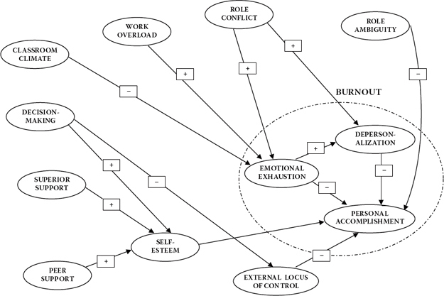
Figure 6.1. Proposed structural model of teacher burnout.

The paths (and their associated signs) leading from the organizational (role ambiguity, role conflict, work overload, classroom climate, decision making, superior support, and peer support) and personality (self-esteem and external locus of control) constructs to the three dimensions of burnout reflect findings in the literature.² For example, high levels of role conflict are expected to cause high levels of emotional exhaustion; in contrast, high (i.e., good) levels of classroom climate are expected to generate low levels of emotional exhaustion.

In viewing the model shown in Figure 6.1, we can see that it represents only the structural portion of the full SEM. Thus, before being able to test this model, we need to determine the manner by which each of the constructs in this model is to be measured. In other words, we now need to specify the measurement portion of the model (see Chapter 1). In contrast to the CFA models studied previously, the task involved in developing the measurement model of a full SEM is twofold: (a) to decide on the number of indicators to use in measuring each latent construct, and (b) to identify how the items will be packaged in formulating each indicator variable.

Formulation of Indicator Variables

In the applications examined in Chapters 3 through 5, the formulation of measurement indicators has been relatively straightforward; all examples have involved CFA models and, as such, comprised only measurement models. In the measurement of multidimensional facets of self-concept (see Chapter 3), each indicator variable represented a pairing of the items comprising each subscale designed to measure a particular self-concept facet. In Chapters 4 and 5, our interest focused on the factorial validity of a measuring instrument. As such, we were concerned with the extent to which the individual items loaded onto their targeted factor. Adequate assessment of this specification demanded that each item be included in the model. Thus, each indicator variable represented one item in the measuring instrument under study.

In contrast to these previous examples, formulation of the indicator variables in the present application is slightly more complex. Specifically, multiple indicators of each construct were formulated through the judicious combination of particular items in comprising item parcels. As such, items were carefully grouped according to content in order to equalize the measurement weighting across the set of indicators measuring the same construct (see, e.g., Hagtvet & Nasser, 2004). For example, the Classroom Environment Scale (Bacharach, Bauer, & Conley, 1986), used to measure Classroom Climate, consists of items that tap classroom size, the ability and interest of students, and various types of abuse by students. Indicators of this construct were formed such that each item in the composite measured a different aspect of classroom climate. In the measurement of classroom climate, self-esteem, and external locus of control, all parcels consisted of items from single unidimensional scales; all remaining item parcels derived from subscales of multidimensional scales. (For an extensive description of the measuring instruments, see Byrne, 1994b.) In total, 32 item parcel indicator variables were used to measure the hypothesized structural model, and all were unidimensional in structure. This issue of parcel unidimensionality is an important one as it substantiates our use of parceling in this full SEM application (see Bandalos, 2002, 2008; Sass & Smith, 2006). Figure 6.2 presents this hypothesized full SEM model of burnout.

In the time since the present study was conducted, there has been a growing interest in the question of item parceling. Research has focused on such issues as method of parceling (Bandalos, 2008; Bandalos & Finney, 2001; Hagtvet & Nasser, 2004; Kim & Hagtvet, 2003; Kishton & Widaman, 1994; Little, Cunningham, Shahar, & Widaman, 2002; Rogers & Schmitt, 2004), the number of indicators per factor (Marsh, Hau, Balla, & Grayson, 1998; Nasser-Abu & Wisenbaker, 2006), the extent to which item parcels affect model fit (Bandalos, 2002; Nasser-Abu & Wisenbaker, 2006; Sass & Smith, 2006), the effects of item parcel use with both sample size (Hau & Marsh, 2004; Nasser-Abu & Wisenbaker, 2006) and nonnormal data (Bandalos, 2008; Hau & Marsh, 2004), and, more generally, whether or not researchers should even engage in item parceling at all (Little et al., 2002; Little, Lindenberger, & Nesselroade, 1999). For an excellent summary of the pros and cons of item parceling, see Little et al. (1999); and for a thorough review of issues related to item parceling, see Bandalos and Finney (2001). (For details related to each of these aspects of item parceling, readers are advised to consult these references directly.)

Confirmatory Factor Analyses

Because (a) the structural portion of a full SEM involves relations among only latent variables, and (b) the primary concern in working with a full SEM model is to assess the extent to which these relations are valid, it is critical that the measurement of each latent variable be psychometrically sound. Thus, an important preliminary step in the analysis of full latent variable models is to test first for the validity of the measurement model before making any attempt to evaluate the structural model. Accordingly, CFA procedures are used in testing the validity of the indicator variables. Once it is known that the measurement model is operating adequately, one can then have more confidence in findings related to assessment of the hypothesized structural model.

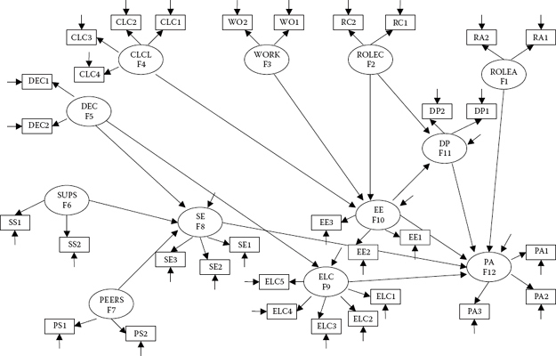
Figure 6.2. Hypothesized SEM model of teacher burnout.

In the present case, CFAs were conducted for indicator variables derived from each of the two multidimensional scales—the Teacher Stress Scale (TSS; Pettegrew & Wolf, 1982) and the Maslach Burnout Inventory (MBI; Maslach & Jackson, 1981, 1986). The TSS comprises six subscales, with items designed to measure Role Ambiguity, Role Conflict, Work Overload, Decision Making, Superior Support, and Peer Support. The MBI, as you know from our work in Chapter 4, comprises three subscales, with items designed to measure three facets of burnout—Emotional Exhaustion, Depersonalization, and (reduced) Personal Accomplishment.

As preanalysis of these data revealed evidence of some nonnormality, all subsequent analyses to be conducted in this chapter are based on robust maximum likelihood (MLM) estimation. CFA results for both the TSS (MLM χ²_[39] = 328.470; Comparative Fit Index [CFI] = .959; Root Mean Square Error of Approximation [RMSEA] = .072; Standardized Root Mean Square Residual [SRMR] = .041) and MBI (MLM χ²_[17] = 148.601; CFI = .970; RMSEA = .074; SRMR = .039) were found to exhibit exceptionally good fit to the data. Nonetheless, examination of the Modification Indices (MIs) for the TSS revealed the freely estimated indicator variable of Decision Making (DEC2) to cross-load significantly onto both Factor 1 (Role Ambiguity) and Factor 5 (Superior Support). Given that these subscales are components of the same measuring instrument, it is not surprising that there may be some overlap of item content across subscales; the CFA model for the TSS was respecified to include these two additional parameters. Results of this analysis yielded a statistically and substantially better fitting model (MLM χ²_[37] = 153.285; CFI = .983; RMSEA = .047; SRMR = .020).

Models of both the revised TSS and the MBI are schematically portrayed in Figure 6.3. It is important that I draw your attention to the numbered labeling of the TSS factors, which you will note are designated as F1, F2, F3, and F5, F6, F7, rather than as F1–F6. My reasoning here was simply to retain consistency with the labeling of these factors in the full SEM model (see Figure 6.2). The TSS retained this revised specification throughout all analyses of the full causal model.

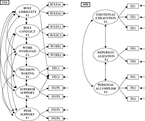
Figure 6.3. Final CFA models of the Teacher Stress Scale (TSS; Pettegrew & Wolf, 1982) and the Maslach Burnout Inventory (MBI; Maslach & Jackson, 1981, 1986).

Mplus Input File Specification and Output File Results

Input File 1

Now that we have established the best fitting and substantively appropriate measurement model, allow me to highlight particular aspects of the input file for the initially hypothesized model as shown in Figure 6.4.

Turning first to the VARIABLE command, we see that all observed variables listed are consistent with those modeled in Figure 6.2. That is, there are no other variables in the model other than the 32 indicator variables listed in the input file. Second, note that an ANALYSIS command is included. The reason for this specification derives from the fact that analyses will not be based on defaulted ML estimation but, rather, on robust MLM estimation in order to address the known nonnormality in the data. Third, consistent with Figure 6.2, the MODEL command comprises two sets of specifications—one set detailing the measurement model (lines 1 to 12), and the other detailing the structural model (lines 13 to 17). Although you likely will have no difficulty in following the specification of most indicator variables, I wish to draw your attention to one in particular, that of DEC2. Recall that, in testing for the validity of factor structure for the TSS in which this variable represents a subscale, we determined that DEC2 exhibited large and statistically significant cross-loadings on Factor 1 (Role Ambiguity) and on Factor 6 (Superior Support). Thus, in addition to its intended loading onto Factor 5 (Decision Making), the indicator variable of DEC2 is shown also to load onto Factors 1 and 6 (circled in Figure 6.4). Fourth, we turn now to specifications related to the structural model. In working through this section, I believe you will find it very helpful if you check each specification against the model itself as shown in Figure 6.2 The first thing you will note with this section of the specifications is use of the word ON, which has not appeared in any of the three previous applications. Nonetheless, in Chapter 2, I explained that the ON statement is short for “regressed on.” Thus, for example, the first structural command specifies that Factor 8 (Self-Esteem) is regressed onto three factors: Factor 5 (Decision Making), Factor 6 (Superior Support), and Factor 7 (Peer Support). In reviewing the model in Figure 6.2, you will readily discern these specified structural paths. Finally, the OUTPUT command requests the reporting of both the MIs and the TECH1 option (for details related to this option, see Chapter 3). My rationale for including the TECH1 option here is that it provides for a check on the extent to which the reported number of degrees of freedom is correct and consistent with our hypothesized model. More specifically, the TECH1 option requests that all freely estimated parameters be presented in array form. Given that these parameters are assigned a number,³ it can assist in determining the expected number of degrees of freedom. Nonetheless, this process is not exactly straightforward in Mplus and will be detailed shortly.

Figure 6.4. Mplus input file for hypothesized model of teacher burnout.

Undoubtedly, you may wonder why I have not requested the standardized solution on the OUTPUT command. In testing for the validity of full SEM models, I prefer to work through all analyses first so that I can establish the final best fitting, albeit most parsimonious, model. Once I have determined this final model, I then request results bearing on the standardized solution.

It is important to mention that although you do not see specifications related to variances of the independent (i.e., exogenous) latent variables in the model (Factors 1 through 7), residuals associated with the observed variables, and residuals with the dependent (i.e., endogenous) latent variables in the model (Factors 8 through 12), these parameters are automatically estimated by default in Mplus (see Muthén & Muthén, 2007-2010). Likewise, covariances among the independent latent variables in the model (Factors 1 through 7) are also estimated by default.

Output File 1

In reviewing this initial output file, results are reported separately for each selected section.

Summary Information

Appearing first in the output is a section detailing the Summary of Analysis; shown in Table 6.1 is a listing of the number of groups (1), observations (N = 1430), all observed and latent variables in the model, as well as other information related to estimation of the model.

Given the complexity of specification related to this application, compared with previous applications thus far, I consider it worthwhile to more fully detail the categorization of all variables in the model to ensure that you fully comprehend the status of each. From my own perspective, I find it easiest to conceptualize all variables in the model (regardless of whether observed or latent) as either dependent or independent variables in the model. As noted previously, independent variables in a model are also termed exogenous variables, whereas dependent variables in a model are termed endogenous variables. Although these latter terms are typically used with respect to latent variables (i.e., factors), they can, of course, also pertain to observed variables. Simplistically, the key defining feature associated with any dependent variable within a causal modeling framework is that it will have one or more single-headed arrows leading to it from other variables in the model; in contrast, all arrows will lead away from independent variables.

Table 6.1 Mplus Output for Hypothesized Model: Summary Information

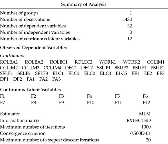
With this simple rule in hand, let's now review the remaining Mplus summary output in Table 6.1. Listed here, we see reported 32 dependent variables and 12 continuous latent variables, followed by their labels. However, because it can be helpful in understanding why certain parameters are not estimated, I prefer to expand on this information in showing that, in fact, the number of variables in the model is as follows:

• 37 dependent variables:

• 32 observed indicators (ROLEA1 to PA3)

• 5 factors (F8–F12)

• 7 independent variables:

• 7 factors (F1–F7)

Appearing next in the output is the warning message shown in Figure 6.5 regarding the latent variable covariance (PSI) matrix.

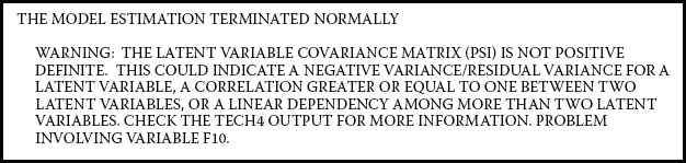
Figure 6.5. Mplus error message concerning input data.

Recall from Chapter 3 that the PSI matrix represents the variance–covariance matrix for the latent factors. Here, it is suggested that the problem may lie with Factor 10 (Emotional Exhaustion). Indeed, not uncommon to full SEM models is the finding of a negative variance related to one of the factors, and this is the case here, as we shall see shortly when we examine the parameter estimates.

Model Assessment

Preceding the reporting of parameter estimates in the Mplus output is a summary of the tests for model fit; these values are reported in Table 6.2. Here we see that the rescaled χ² value (i.e., the MLM χ²) is 1554.942 with 427 degrees of freedom. The reported scaling correction value for the MLM estimator indicates that if the MLM χ² were multiplied by 1.117, it would approximate the uncorrected ML χ² value (1736.870). Indeed, reanalysis of the hypothesized model based on ML estimation certainly approximated this value in yielding a χ² value of 1737.090.

Further on this topic, as noted in both Chapters 4 and 5, whenever robust parameter estimation is used, chi-square difference tests between nested models are inappropriate because the chi-square-difference values are not distributed as chi-square. These tests, however, can still be conducted, albeit using the correction formula reported in a paper by Satorra and Bentler (2001) that is also available on the Mplus website (http://www.statmodel.com/chidiff.shtml). Accordingly, results based on robust estimation are always accompanied by a caveat in the Mplus output as shown in Table 6.2.

Table 6.2 Mplus Output for Hypothesized Model: Selected Goodness-of-Fit Statistics

Tests of Model Fit
Chi-Square Test of Model Fit
Value	1554.942*
Degrees of freedom	427
p-value	0.0000
Scaling Correction Factor for MLM	1.117
CFI/TLI
CFI	0.945
TLI	0.936
Number of free parameters	133
Root Mean Square Error of Approximation (RMSEA)
Estimate	0.043
Standardized Root Mean Square Residual (SRMR)
Value	0.051

* The chi-square value for MLM, MLMV, MLR, ULSMV, WLSM, and WLSMV cannot be used for chi-square difference testing in the regular way. MLM, MLR, and WLSM chisquare difference testing is described on the Mplus website (http://www.statmodel.com). MLMV, WLSMV, and ULSMV difference testing is done using the DIFFTEST option.

As indicated by the CFI and Tucker-Lewis Fit Index (TLI) values of 0.945 and 0.936, respectively, the hypothesized model exhibits a relatively good fit to the data. Reported values of both the RMSEA (0.043) and SRMR (0.051) provide additional support in this regard. Nonetheless, examination of the MIs will enable us to refine this initial model assessment.

Earlier in this chapter, in my review of the Mplus input file, I noted that inclusion of the TECH1 option in the OUTPUT command can be helpful in determining if the number of reported estimated parameters and, ultimately, the number of degrees of freedom are correct as this information can alert you to whether or not the model is correctly specified. Thus, prior to moving on to an examination of the parameter estimates, I wish first to digress slightly in order to review several related important points. To aid us in this process, we turn to the selected portions of the TECH1 output reported in Figure 6.6.

Although results pertinent to only the BETA and PSI matrices are included here, the information provided is sufficient for our immediate purposes. First, I noted earlier that the TECH1 option presents matrix-formatted arrays of all freely estimated parameters in the model; accordingly, each parameter is assigned a number. In the BETA matrix, for example, you will note that the numbers range from 87 through 100. The 14 numbers assigned to parameters in this matrix represent the 14 structural paths to be estimated in the model. In the F1 column, for example, the number 96 is the number assigned to the parameter representing the path leading from Factor 1 to Factor 12.

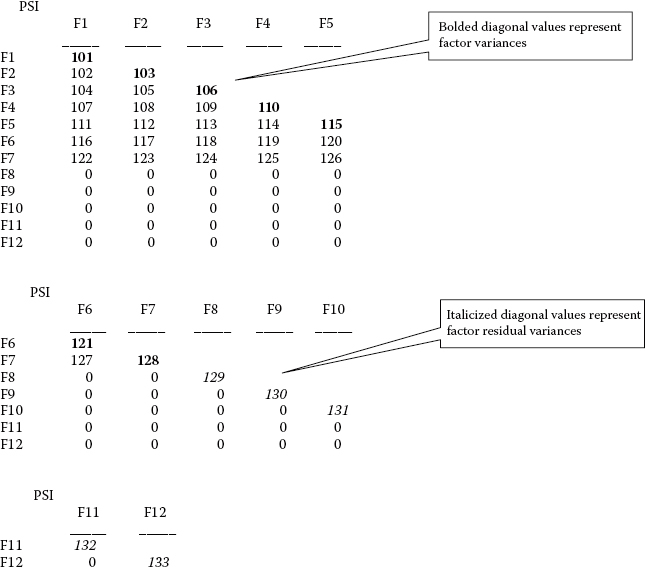
Second, turning next to the PSI matrix, we find estimated parameters on both its diagonal and a portion of its off-diagonals. As noted in the callouts in this table, the bolded numbers on the diagonal represent the variances of Factors 1 through 7, whereas the italicized numbers on the lower section of the diagonal represent the residuals associated with Factors 8 through 12. Why the difference between the two sets of factors? Recall from Chapter 2 that one important tenet of SEM is that the estimation of variances and covariances is pertinent to only the independent variables in a model. Thus, only the variances of Factors 1 through 7 are estimated. In contrast, the variances for Factors 8 through 12 actually represent their residuals as these latter parameters, technically speaking, are independent parameters in the model. Likewise, the 21 factor covariances estimated represent those among Factors 1 through 7.

Third, note that the variance of the residual associated with Factor 12 represents the final parameter to be estimated, and note also that it is assigned the number 133. Thus, according to the Mplus TECH1 output, there are 133 parameters to be estimated for the hypothesized model. (See also the number of free parameters noted in the section of the output file reported in Table 6.2.) Recall that by default, Mplus always estimates the intercepts for the observed variables, and, therefore, this number is correctly reported in Table 6.2. However, given that we are working within the framework of covariance, rather than mean structure modeling, the observed variable means (i.e., intercepts) are of no interest, and, thus, the program automatically fixes these values to 0.0. As a consequence, the actual number of estimated parameters is 101 (133 - 32), and not 133, given that there are 32 observed variables and, hence, 32 intercepts.

Finally, recall that in Chapter 2, I explained how to calculate the number of degrees of freedom associated with a specified model. At that time, I introduced you to the formula p (p + 1)/2, where p represents the number of observed variables in a specified model. I also noted at that time that, because Mplus estimates the observed variable intercepts by default, additional pieces of information must necessarily include the observed variable means. Thus, the complete formula is p (p + 1)/2 + p means. Calculations based on this formula yield the number of elements (or moments; i.e., pieces of information) upon which analyses will be based; this resulting number minus the number of estimated parameters equals the number of degrees of freedom. However, as noted previously, when SEM analyses are based on covariance rather than on mean structures, the factor mean estimates are fixed to zero by default and the number of observed variable intercepts is not included in calculations of degrees of freedom. With this information in hand, then, let's now review the number of estimated parameters in our hypothesized model and then calculate the number of expected degrees of freedom.

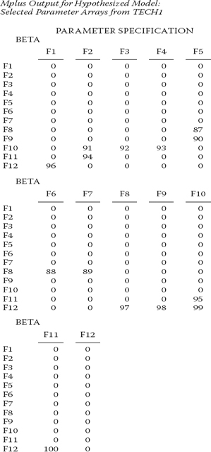
Figure 6.6. Mplus parameter arrays resulting from TECH1 specification in OUTPUT command.

• 101 estimated parameters:
22 factor loadings (20 original and 2 additional)
44 variances (7 factors, 32 error residuals, and 5 factor residuals)
21 factor covariances (Factors 1–7)
14 structural regression paths

• 528 pieces of information:
Number of observed variables = 32
p (p + 1)/2

= 32 (32 + 1)/2

= 32 (33)/2

= 1056/2 = 528

• 427 degrees of freedom (528 - 101)

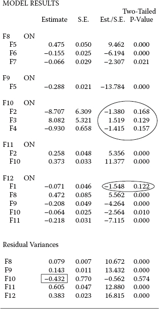
Figure 6.7. Mplus output showing structural regression path and residual variance estimates.

A quick comparison with the results reported in Table 6.2 reveals this number of degrees of freedom to be correct.

Model Parameter Estimation

Given the large number of parameters estimated in this model, the reported results are understandably lengthy. Thus, in the interest of space, I report findings pertinent to only the structural parameters, as well as a few residual variances. These results are presented in Figure 6.7.

Examination of estimated parameters in the model revealed all to be statistically significant except for five as reported in Figure 6.7. Four of these nonsignificant parameters are shown within ovals and represent the following structural regression paths: (a) F10 on F2 (Role Conflict → Emotional Exhaustion), F10 on F3 (Work Overload → Emotional Exhaustion), F10 on F4 (Classroom Climate → Emotional Exhaustion), and (b) F12 on F1 (Role Ambiguity → Personal Accomplishment). In my writings, I have stressed that final models in SEM should represent the best fitting, albeit most parsimonious, model of any set of tested models. As such, all parameters in the model must be statistically significant. However, at this point in our testing of the hypothesized model, it is not yet known whether we will need to conduct post hoc analyses in order to further refine the model. Thus, because MI values can fluctuate widely during the process of these post hoc analyses, it is more appropriate to first determine the best fitting model. Once this final model is established, then we can conduct a final model in which any nonsignificant parameters in the model are deleted. Thus, these nonsignificant structural parameters will remain in the model until we have determined our final model.

Let's turn now to estimates of the factor residual variances, also included in Figure 6.7. Pertinent to the warning message noted earlier regarding the nonpositive status of the PSI matrix, we can now see the source of the problem as being a negative variance for the residual associated with Factor 10. It seems likely that this variance is close to zero and, as a boundary parameter, can just as easily be a negative as a positive value. Interpreted literally, this finding implies that the combination of Role Conflict (F2), Work Overload (F3), and Classroom Climate (F4) is perfect in its prediction of Emotional Exhaustion (F10), thereby resulting in no residual variance. However, in the testing of full structural equation models such as the one in this chapter, post hoc model fitting often results in a solution in which the negative variance disappears, which, as you will see later in this chapter, turns out to be the case in the present application.

Model Misspecification

Over and above the fit of our hypothesized model as a whole, which we noted to be relatively good (CFI = .945; TLI= .936), a review of the MIs reveals some evidence of misfit in the model. Because we are interested solely in the causal paths of the model at this point, only MIs related to these parameters are included in Table 6.3.⁴ The Mplus output reports these results in the form of ON/BY, rather than as just ON statements; for each pair, the ON statement, of course, represents the opposite of the BY statement. For example, turning to the first result in Table 6.3, we can recognize that F2 on F8 is the reverse of F8 by F2. Thus, whereas F2 on F8 conveys the notion that F2 is regressed on F8 (i.e., follow the point of the single-headed arrow [at F2] backward to its source [F8]), the statement F8 by F2 signals that F2 is influenced by F8 (i.e., the arrow points from F8 to F2). Accompanying the reported MI estimate associated with each ON/BY statement is the expected parameter change (EPC) statistic, along with its standardized values. We turn now to these results in Table 6.3.

Table 6.3 Mplus Output for Hypothesized Model: Selected Modification Indices (MIs)

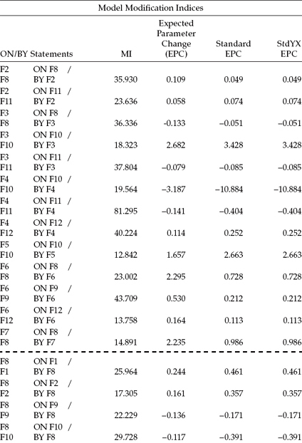
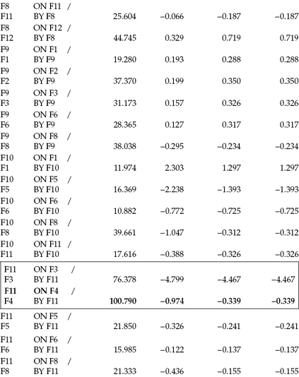
Given that the primary research focus bearing on the current model is to identify determinants of teacher burnout, only paths leading from the independent factors in the model (F1 through F7) to the dependent factors (F8 through F12) qualify as candidates for inclusion in subsequent models. Thus, although we may find MIs related to paths leading from dependent to independent factors or the presence of reciprocal paths, these parameters are not considered with respect to the current research and model. The dotted line shown in Table 6.3 serves to separate most (but not all) MIs related to paths flowing in the desired direction (independent to dependent) from those flowing from dependent to independent factors.

In reviewing the ON/BY statements below the dotted line, you will note that two are encased within a rectangle. Focusing on these captured values, we see that the maximum MI (bolded text) is associated with the regression of F11 on F4 (Depersonalization on Classroom Climate). The value of 100.790 indicates that, if this parameter were to be freely estimated in a subsequently specified model, the overall χ² value would drop by at least this amount. The EPC statistic related to this parameter is shown to be -0.974; this value represents the approximate value that the newly estimated parameter would assume. The negative sign associated with this value is substantively correct and as expected, given that items from the Classroom Environment Scale were reflected such that low scores were indicative of a poor classroom milieu, and high scores of a good classroom milieu.

The other ON/BY statement (F11 on F3) within the rectangle is included here as it provides me with an opportunity to stress the importance of selecting potentially additional model parameters only on the basis of their substantive meaningfulness. Given the noticeably high MI associated with this structural path and its exceptionally high EPC value, a researcher might consider the selection of this parameter over the previous one. Indeed, there has been some suggestion in the literature that the selection of post hoc parameters on the basis of their EPCs may be more appropriate than on the basis of their MIs (see, e.g., Kaplan, 1989; but see Bentler's [2005] caveat that these values can be affected by both the scaling and identification of factors and variables). However, let's take a closer look at this parameter representing the regression path leading from F3 (Work Overload) to F11 (Depersonalization). That the EPC value is negative is a clear indication that this parameter is inappropriate as this would be interpreted to mean that high Work Overload would lead a teacher to exhibit low levels of Depersonalization, which clearly runs counter to both burnout theory and practical sense.

From a substantive perspective, it would seem perfectly reasonable that secondary teachers whose responses yielded low scores for Classroom Climate should concomitantly display high levels of Depersonalization. Given the meaningfulness of this influential flow, we now proceed within a post hoc modeling framework to reestimate the model, with the path from Classroom Climate to Depersonalization (F11 on F4) specified as a freely estimated parameter; this model is subsequently labeled as Model 2. Results derived from this respecified model are subsequently discussed within the framework of post hoc analyses. I wish once again to stress two important caveats with respect to the post hoc model-fitting process: (a) Once the hypothesized model has been rejected, as we have done here, we are no longer working within a confirmatory framework, and from now on these analyses are of an exploratory nature; and (b) when identification of misspecified parameters is based on the MI, it is critical that any respecification of the model include the addition of only one parameter at a time.

In the post hoc model fitting of full structural equation models in general, and the application included here in particular, the process can be very tedious and time-consuming. Thus, I am certain that you will find this to be the case in this chapter. However, I consider it important to walk you through each and every step in determining the various post hoc models as this, in essence, is really the only way to fully appreciate what is involved in the selection of the various additional parameters to be included in the model.

Post Hoc Analyses

Output File 2

In the interest of space, only portions of the MI results pertinent to each respecified model will be presented in table form; other relevant results are presented and discussed in the text.

Model Assessment

The estimation of Model 2 yielded an overall MLM χ²₍₄₂₆₎ value of 1450.985 (scaling correction factor = 1.117); CFI and TLI values of 0.950 and 0.941, respectively; a RMSEA value of 0.041; and a SRMR value of 0.046. It is important to note that throughout the post hoc analyses, assessment and reporting of the extent to which reestimated models improved model fit were determined from chi-square-difference values (MLMΔχ²) that were, in turn, recalculated on the basis of the correction formula provided in the Mplus website (http://www.statmodel.com) for use with robust estimation. Although improvement in model fit for Model 2, compared with the originally hypothesized model, would appear to be somewhat minimal on the basis of the CFI, TLI, RMSEA, and SRMR values, this decision was ultimately based on the corrected chi-square difference test, which in this case was found to be statistically significant (MLMΔχ²_[1] = 104.445). To provide you with a clear understanding of how this value was derived, I consider it important to walk you through the most relevant stages of this three-step process, as presented in the Mplus website; these comprise the following:

• Computation of the scaling correction factors
• Computation of scaling correction associated with the difference test
• Computation of the MLMχ²–difference test

Given that the scaling correction factors are provided by the Mplus program, there is no need to work through the first step. Thus, for this first comparison model, I illustrate only Steps 2 and 3 as follows:

Step 2. cd = (d0 * c0) – (d1 * c1)/(d0 – d1)

where d0	=	degrees of freedom for the nested (i.e., more restricted) model;
d1	=	degrees of freedom for the comparison (i.e., less restricted) model;
c0	=	scaling correction factor for the nested model (see Table 6.2);
c1	=	scaling correction factor for the comparison model (see text);
cd	=	(427 * 1.117) - (426 * 1.117)/(427 - 426)
	=	(476.959 - 475.842)/1
	=	1.117

That the scaling correction factor for the difference test is 1.117, of course, is not unexpected, given that this value was reported to be the same for both the hypothesized model (Model 1) and Model 2.

Step 3. TRd = (T0 – T1)/cd

where TRd	=	MLM χ2-difference test;
T0	=	ML χ2 for the nested model;5
T1	=	ML χ2 for the comparison model;
TRd	=	(1737.090 - 1620.425)/1.117
	=	116.665/1.117
	=	104.445

Given a reasonably good fit of the model to the data, and the fact that respecification of Model 2 yielded little difference in fit indices from those of the hypothesized model, you may wonder at this point (and rightly so) why we should continue in the search for a better fitting model via specification of additional parameters to the model. The answer to this query is tied to the fact that we are working toward the validation of a full SEM model where the key parameters represent causal structure among several latent constructs. Clearly, our overall aim is to determine the best fitting, albeit most parsimonious, model in representing the determinants of burnout for secondary teachers. Thus, the thrust of these post hoc analyses is to fine-tune our hypothesized structure such that it includes all viable and statistically significant structural paths (which it is here: ΔMLM χ²_[1] = 104.445), and, at the same time, eliminates all nonsignificant paths. Consequently, as long as the Δχ²–difference test is statistically significant, and the newly added parameters are substantively meaningful, I consider the post hoc analyses to be appropriate.

Model Parameter Estimation

Importantly, the estimated value of the path from Classroom Climate to Depersonalization was found to be both statistically significant (-9.643) and exceptionally close to the one predicted by the EPC statistic (-0.969 versus -0.974). Of substantial import is the fact that (a) the warning message noted and described earlier regarding Factor 10 (Emotional Exhaustion) and its negative residual variance remained in the output for Model 2, and (b) the estimated structural regression paths for the three factors hypothesized to influence Factor 10 (Factors 2, 3, and 4) remained statistically nonsignificant.

Modification Indices

All MIs related only to the structural regression parameters for Model 2 are shown in Table 6.4. Consistent with Table 6.3, all ON/BY statements appearing above the broken line represent structural regression paths that run counter to expected direction and therefore are not of interest here. Again, although some inappropriate directional paths appear below this line, most are eligible for consideration in our search for improvement to model fit. In a review of the eligible MIs, I determined the one appearing in the solid rectangle to be most appropriate both substantively and statistically. In addition to having the largest MI (based on appropriate causal direction), it also has a substantial EPC value. This parameter represents the regression of Factor 12 (Personal Accomplishment) on F5 (Decision Making) and suggests that the greater the opportunity for secondary teachers to participate in decision making with respect to their work environment, the stronger will be their sense of personal accomplishment. On the basis of this rationale, I consider it acceptable to once again respecify the model with this new structural path included (Model 3).

Table 6.4 Mplus Output for Model 2: Selected Modification Indices (MIs)

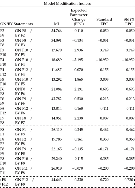
Before leaving these MI results for Model 2, however, I direct your attention to the MI results appearing within the broken rectangle. Given that the MI value is larger than the one I selected, some readers may wonder why I didn't choose the parameter represented here. The explanation relates to the causal direction associated with this parameter as it represents the regression of Factor 8 (Self-Esteem) on F12 (Personal Accomplishment). Although, admittedly, a flow of causal direction from Personal Accomplishment to Self-Esteem is logically possible, it runs counter to the focus of the present intended research in identifying determinants of teacher burnout. On this basis, then, it does not qualify here for considered addition to the model.

Output File 3

Model Assessment

Model 3 yielded an overall MLM χ²₍₄₂₅₎ value of 1406.517 (scaling correction factor = 1.117), with CFI = 0.952, TLI = 0.944, RMSEA = 0.040, and SRMR = 0.044. Again, the MLM χ² difference between Models 2 and 3 is statistically significant ΔMLM χ²_[1] = 44.277), albeit differences in the other fit indices across Models 2 and 3 were once again minimal.

Model Parameter Estimation

As expected, the estimate for the newly incorporated path from Decision Making to Personal Accomplishment (F5 → F12) was found to be statistically significant. Also of interest is the finding that only two of the three previous paths leading to F10 (F2 and F4) are nonsignificant. Furthermore, the structural path leading from F1 (Role Ambiguity) to F12 (Personal Accomplishment) is now statistically significant, albeit the path from F10 to F12 is not so. These dramatic shifts in the parameter estimate results represent a good example of why it is important to include only one respecified parameter at a time when working with univariate MIs in post hoc analyses.⁶ Finally, once again the negative variance associated with the F10 residual was retained, hence the related warning message.

Modification Indices

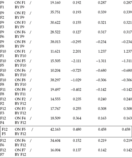
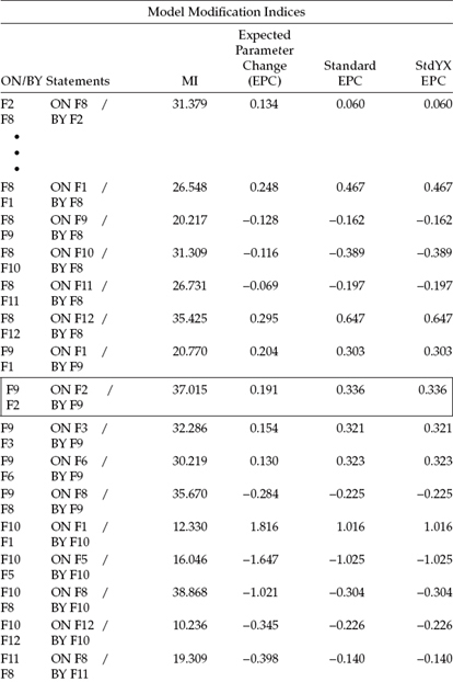
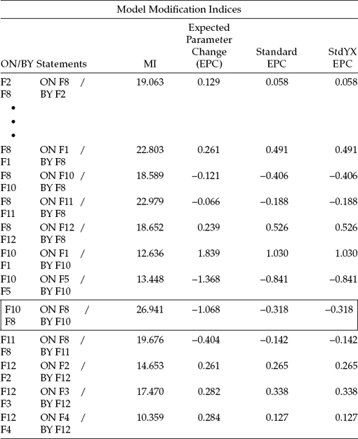
MIs related to Model 3 are presented in Table 6.5. Because the first reasonable MI to be considered is once again F8 on F1, I have chosen to delete all MIs between this one and the first one reported in the output file. Following a review of all remaining MIs, the one considered most appropriate for inclusion in a subsequent model is the structural path flowing from F2 (Role Conflict) to F9 (External Locus of Control). Thus, information related to the MI representing this parameter is shown within the rectangle.

Again, I believe it is worthwhile to note why two alternate MI values, close in value to the one chosen here, are considered to be inappropriate. I refer to results related to the structural paths of F10 on F8 (MI = 38.868) and of F9 on F8 (MI = 35.670). In both cases, the flow of causal direction is incorrect. In contrast, the structural path noted earlier (F9 on F2) is viable both statistically and substantively in that high levels of role conflict can be expected to generate high levels of external locus of control, thereby yielding a positive EPC statistic value, which is the case here (EPC = 0.191). Thus, Model 4 was subsequently specified with the path leading from Role Conflict to External Locus of Control (F9 on F2) freely estimated.

Output File 4

Model Assessment

The estimation of Model 4 yielded a MLM χ² value of 1366.129 (scaling correction factor = 1.118) with 424 degrees of freedom. Values related to the CFI, TLI, RMSEA, and SRMR were .954, .946, 0.039, and 0.041, respectively. Again, the difference in fit between this model (Model 4) and its predecessor (Model 3) was statistically significant (MLMΔχ²_[1] = 63.782).

Model Parameter Estimation

As expected, the newly specified parameter (F9 on F2) was found to be statistically significant (Estimate = 0.189; Estimate [Est]/standard error [SE] = 7.157). However, once again the three paths leading from F2, F3, and F4 to F10 were all found to be nonsignificant, in addition to yet another different path leading to F12—that of F12 on F10 (Emotional Exhaustion → Personal Accomplishment). Finally, once again, the warning message regarding the negative residual associated with Factor 10 appeared in the output file.

Table 6.5 Mplus Output for Model 3: Selected Modification Indices (MIs)

Modification Indices

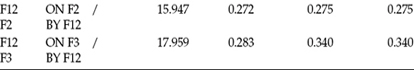
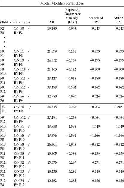
MIs related to the estimation of Model 4 are presented in Table 6.6. Once again, I have deleted all ineligible MI values appearing between the first appropriate result (F8 on F1) and the first MI result specified in the output (F2 on F8). As usual, the parameter that I consider most appropriate for inclusion in the model is encased within a rectangle; in the case of Model 4, it represents the structural regression path from Factor 8 (Self-Esteem) to Factor 9 (External Locus of Control). This parameter represents the largest by far of all MI estimates that qualify for inclusion in a subsequent model; and, again, it is substantively meaningful because, clearly, the lower a teacher's sense of self-esteem, the more he or she is going to feel under the control of others. Thus, we move on to Model 5, in which this parameter has been included in the model.

Output File 5

Model Assessment

The estimation of Model 5 yielded a MLM χ²₍₄₂₃₎ value of 1331.636 (scaling correction factor = 1.117), with other fit indices as follows: CFI = 0.955, TLI = 0.948, RMSEA = 0.039, and SRMR = 0.039. Again, the difference in fit between this model (Model 5) and its predecessor (Model 4) was found to be statistically significant (S-BΔχ²_[1] = 25.410).

Model Parameter Estimation

Once again, the newly specified parameter (F9 on F8) was found to be statistically significant and accompanied by the correct sign (Estimate = 0.257; Est/SE = 5.337). However, as with Model 3, again two of the three paths leading to F10 (F2 → F10; F4 → F10) remained statistically nonsignificant, albeit the third previously nonsignificant path now yielded a significant estimated value. Finally, the path leading from F10 (Emotional Exhaustion) to F12 (Personal Accomplishment) remained statistically nonsignificant, and the warning message regarding the negative residual associated with Factor 10 remained unchanged.

Table 6.6 Mplus Output for Model 4: Selected Modification Indices (MIs)

Modification Indices

MIs related to the estimation of Model 5 are presented in Table 6.7. This output file reveals the structural path leading from Self-Esteem to Emotional Exhaustion (F8 → F10) as having the largest MI value. Because Factor 10 has been problematic regarding the estimation of its residual in yielding a negative variance, it would seem likely that if this parameter were to be included in the model, this undesirable result may finally be resolved. Thus, given that the related EPC statistic related to this parameter exhibits the correct sign, together with the fact that it seems reasonable that teachers who exhibit high levels of self-esteem may, concomitantly, exhibit low levels of emotional exhaustion, the model was reestimated once again, with this path freely estimated (Model 6).

Selected Mplus Output: Model 6

Model Assessment

The estimation of Model 6 yielded a MLM χ²₍₄₂₂₎ value of 1297.489 (scaling correction factor = 1.116), with the remaining fit indices as follows: CFI = 0.957, TLI = 0.949, RMSEA = 0.038, and SRMR = 0.039. As might be expected given the newly specified path involving Factor 10, the difference in fit between this model (Model 6) and its predecessor (Model 5) was found to be statistically significant (MLMΔχ²_[1] = 39.973).

Model Parameter Estimation

Perhaps the most interesting finding here is that the warning message concerning Factor 10 no longer appeared in the output file as the negative residual variance associated with this factor had now been eliminated. As expected, the estimated value for the newly specified path (F10 on F8) was statistically significant (Estimate = -0.884; Est/SE = -8.116). Interestingly, the previously determined nonsignificant paths loading onto F10 (F2, F3, F4), were all statistically significant. Nonetheless, the regression path leading from F10 to F12, which has been consistently nonsignificant, remained so. In addition, however, the parameter, F8 on F7 (Peer Support → Self-Esteem), was found to be statistically nonsignificant.

Table 6.7 Mplus Output for Model 5: Selected Modification Indices (MIs)

Modification Indices

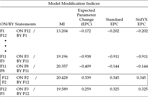
Of the two highest MIs reported in Table 6.8 (F11 on F8; F12 on F2), only the latter one makes sense substantively; this parameter is highlighted within the rectangle. More specifically, the first parameter represents a causal path flowing from F8 (Self-Esteem) to F11 (Depersonalization). However, the fact that the EPC statistic has a negative sign makes interpretation of this path illogical as it conveys the notion that high self-esteem leads to low levels of depersonalization; more appropriately, the path should have a positive sign. In contrast, the positive sign associated with the path leading from Role Conflict to Personal Accomplishment does make sense as this construct actually represents a sense of reduced personal accomplishment. Thus, I consider it worthwhile to specify one more model (Model 7) that incorporates this parameter (F12 on F2).

Table 6.8 Mplus Output for Model 6: Selected Modification Indices (MIs)

Output File 7

Model Assessment

The estimation of Model 7 yielded a MLM χ²₍₄₂₁₎ value of 1277.061 (scaling correction factor = 1.115), with the remaining fit indices as follows: CFI = 0.958, TLI = 0.950, RMSEA = 0.038, and SRMR = 0.038. Again, the difference in fit between this model (Model 7) and its predecessor (Model 6) was found to be statistically significant (MLMΔχ²_[1] = 15.149).

Model Parameter Estimation

Here again, the new parameter added to the model (F12 on F2) was found to be statistically significant (Estimate = 0.332; Est/SE = 4.736). However, the structural regression paths F8 (Self-Esteem) on F7 (Peer Support), and F12 (Personal Accomplishment) on F1 (Role Ambiguity), remained the only two statistically nonsignificant parameters in the model.

At this point, I believe that we have exhausted the search for a better fitting model that best represents the data for secondary teachers. Thus, I do not include a section dealing with the MIs. Rather, I suggest that we move on to the establishment of an appropriate final model. Up to this point in the post hoc modeling process, we have focused on only the addition of parameters to the model, all of which were found to be justified from both a statistical and a practical perspective. Now we need to look at the flip side of the coin in identifying all paths that were originally specified in the hypothesized model but remain statistically nonsignificant as per the results for Model 7; these parameters need to be deleted from the model. Accordingly, Model 8 is now specified in which the two nonsignificant parameters noted above (F7 → F8; F1 → F12) are not included. This model will represent our final best fitting and most parsimonious model of burnout for secondary teachers. Because standardized estimates are typically of interest in presenting results from structural equation models, I have included this requested information on the OUTPUT command. The input file for this final model is shown in Figure 6.8.

Output File 8 (Final Model)

As Model 8 represents the final model, key components of the output files are presented in tabled form. We begin, as usual, with the goodness-of-fit results.

Model Assessment

As shown in Table 6.9, estimation of this final model (Model 8) yielded an overall MLM χ²₍₄₂₃₎ value of 1277.333 (scaling correction factor = 1.116). Of course, the reason for the additional two degrees of freedom, compared with the previously tested model (Model 7), derives from the deletion of the two structural regression paths. As you can readily determine from the CFI value of 0.958, this final model represents a very good fit to the data for secondary teachers. The remaining TLI, RMSEA, and SRMR values further substantiate these results. In contrast to all previous models tested here, we can expect the corrected chi-square difference between the present model and Model 7 to be statistically nonsignificant given that the two parameters deleted in this model were already found to be statistically nonsignificant in Model 7. Indeed, this was the case as the corrected Δχ²₍₂₎ value was found to be 3.371.

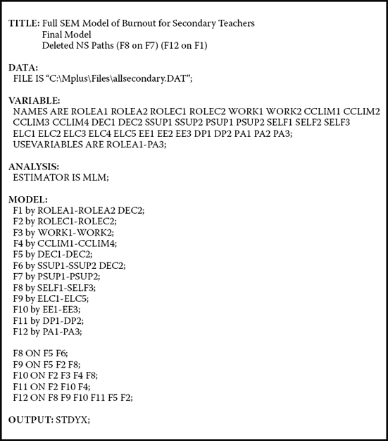
Figure 6.8. Mplus input file for final model of teacher burnout for secondary teachers.

Table 6.9 Mplus Output for Model 8 (Final Model): Selected Goodness-of-Fit Statistics

Tests of Model Fit
Chi-Square Test of Model Fit
Value	1277.333*
Degrees of freedom	423
p–value	0.0000
Scaling Correction Factor for MLM	1.116
CFI/TLI
CFI	0.958
TLI	0.951
Root Mean Square Error of Approximation (RMSEA)
Estimate	0.038
Standardized Root Mean Square Residual (SRMR)
Value	0.038

Model Parameter Estimation

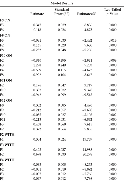
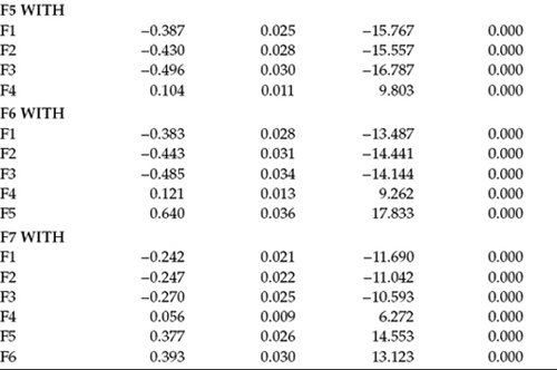
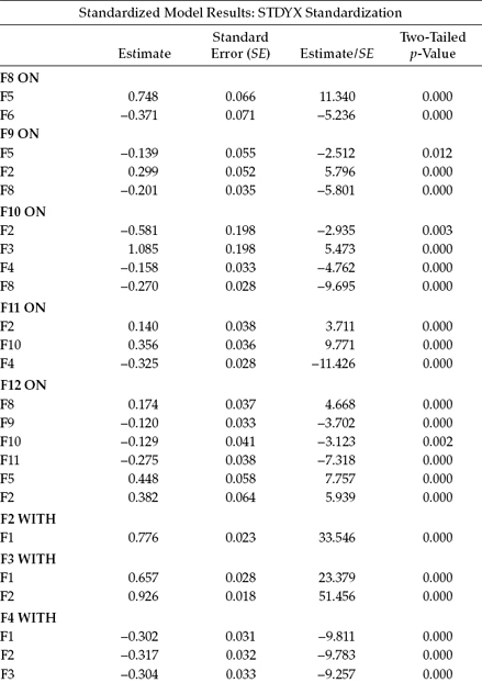
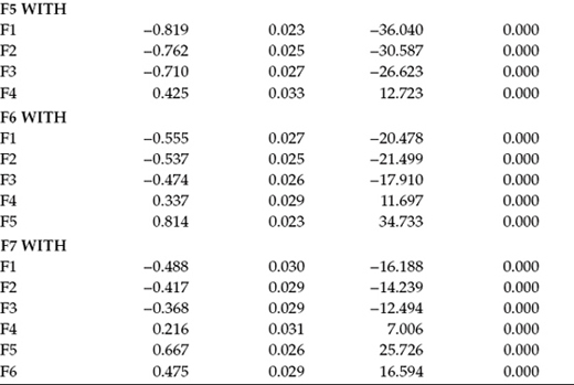
Although all estimated parameters were statistically significant, space restrictions prevent me from presenting them all in the table. Thus, reported in Table 6.10 are the unstandardized estimates pertinent to only the structural regression paths and the factor covariances. The standardized estimates are presented in Table 6.11.

In a review of the standardized estimates, I draw your attention to the WITH statements and subsequently to one disturbingly high correlation of 0.926 between F3 (Work Overload) and F2 (Role Conflict). That both constructs represent subscales from the same measuring instrument (TSS), however, is not surprising and suggests that the items in one or both scales contain content that may not be clearly specific to its targeted underlying construct. A subsequent respecification of this burnout model might benefit from the inclusion of only one of these two constructs, albeit using all four indicators in its measurement (see, e.g., Chapter 9). A schematic representation of this final model is shown in Figure 6.9.

In working with structural equation models, it is very important to know when to stop fitting a model. Although there are no firm rules or regulations to guide this decision, the researcher's best yardsticks include (a) a thorough knowledge of the substantive theory, (b) an adequate assessment of statistical criteria based on information pooled from various indices of fit, and (c) a watchful eye on parsimony. In this regard, SEM researcher must walk a fine line between incorporating a sufficient number of parameters to yield a model that adequately represents the data, and falling prey to the temptation of incorporating too many parameters in a zealous attempt to attain the statistically best fitting model. Two major problems with the latter tack are that (a) the model can comprise parameters that actually contribute only trivially to its structure, and (b) the more parameters a model contains, the more difficult it is to replicate its structure should future validation research be conducted.

Table 6.10 Mplus Output: Selected Model Unstandardized Parameter Estimates

In bringing this chapter to a close, it may be instructive to summarize and review findings from the various models tested in this full SEM application. A visual summary of both the original and post hoc–added structural paths is presented in Figure 6.10. First, of the 14 structural regression paths specified in the hypothesized model (see Figure 6.2), 10 were found to be statistically significant for secondary teachers. These paths reflected the impact of (a) decision making, superior support, and peer support on the self-esteem; (b) decision making on external locus of control; (c) role conflict and emotional exhaustion on depersonalization; and (d) self-esteem, external locus of control, emotional exhaustion, and depersonalization on reduced personal accomplishment. Second, six structural paths, not specified a priori, proved to be essential components of the causal structure and therefore were added to the model. These paths were (a) Role Conflict → Personal Accomplishment, (b) Role Conflict → External Locus of Control, (c) Classroom Climate → Depersonalization, (d) Decision Making → Personal Accomplishment, (e) Self-Esteem → Emotional Exhaustion, and (f) Self-Esteem → External Locus of Control. Finally, two originally hypothesized paths (Role Ambiguity → Personal Accomplishment; Peer Support → Self-Esteem) were found not to be statistically significant and were therefore deleted from the model. As a consequence of these deletions, the constructs of Role Ambiguity and Peer Support became redundant and were also removed from the model.⁷

Table 6.11 Mplus Output: Selected Standardized Parameter Estimates

In conclusion, based on our analyses of this full SEM application, it seems evident that role conflict, work overload, classroom climate, (the opportunity to participate in) decision making, and the support of one's superiors are potent organizational determinants of burnout for high school teachers. However, the process appears to be tempered by one's general sense of self-esteem and locus of control.

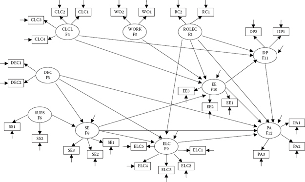
Figure 6.9. Final model of burnout for secondary teachers.

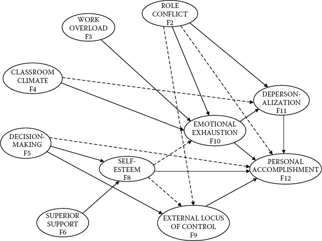
Figure 6.10. Summary of final model structural paths representing determinants of burnout for secondary teachers. Note: Solid arrows represent originally hypothesized regression paths; broken arrows represent regression paths added to model following tests of its validity.

Notes

1.	More correctly, the PA factor actually represents reduced PA.
2.	To facilitate interpretation, particular items were reflected such that high scores on role ambiguity, role conflict, work overload, EE, DP, and external locus of control represented negative perceptions, and high scores on the remaining constructs represented positive perceptions.
3.	The assignment of numbers is primarily for purposes of parameter identification in error messages pertinent to model nonidentification and other uses.
4.	The reasoning here is because in working with full structural equation models, any misfit to components of the measurement model should be addressed when that portion of the model is tested for its validity. Indeed, this approach is consistent with our earlier work in this chapter.
5.	The ML χ2 values are obtained from separate analyses of the two models based on ML estimation.
6.	In contrast, for example, the Lagrange Multiplier Test used in the EQS program utilizes a multivariate approach to testing for evidence of misspecification.
7.	Although not included here, but illustrated in Chapter 9, in order to portray this final model more appropriately, it should be restructured with the assignment of factor numerals revised accordingly.