chapter 3

Testing the Factorial Validity
of a Theoretical Construct

First-Order Confirmatory
Factor Analysis Model

Our first application examines a first-order confirmatory factor analysis (CFA) model designed to test the multidimensionality of a theoretical construct. Specifically, this application tests the hypothesis that self-concept (SC), for early adolescents (grade 7), is a multidimensional construct composed of four factors—General SC (GSC), Academic SC (ASC), English SC (ESC), and Mathematics SC (MSC). The theoretical underpinning of this hypothesis derives from the hierarchical model of SC proposed by Shavelson, Hubner, and Stanton (1976). The example is taken from a study by Byrne and Worth Gavin (1996) in which four hypotheses related to the Shavelson et al. model were tested for three groups of children—preadolescents (grade 3), early adolescents (grade 7), and late adolescents (grade 11). Only tests bearing on the multidimensional structure of SC, as it relates to grade 7 children, are relevant in the present chapter. This study followed from earlier work in which the same four-factor structure of SC was tested for adolescents (see Byrne & Shavelson, 1986) and was part of a larger study that focused on the structure of social SC (Byrne & Shavelson, 1996). For a more extensive discussion of the substantive issues and the related findings, readers should refer to the original Byrne and Worth Gavin article.

The Hypothesized Model

In this first application, the inquiry focuses on the plausibility of a multidimensional SC structure for early adolescents. Although such dimensionality of the construct has been supported by numerous studies for grade 7 children, others have counterargued that SC is less differentiated for children in their pre- and early adolescent years (e.g., Harter, 1990). Thus, the argument could be made for a two-factor structure comprising only GSC and ASC. Still others postulate that SC is a unidimensional structure, with all SC facets embodied within a single SC construct (GSC).

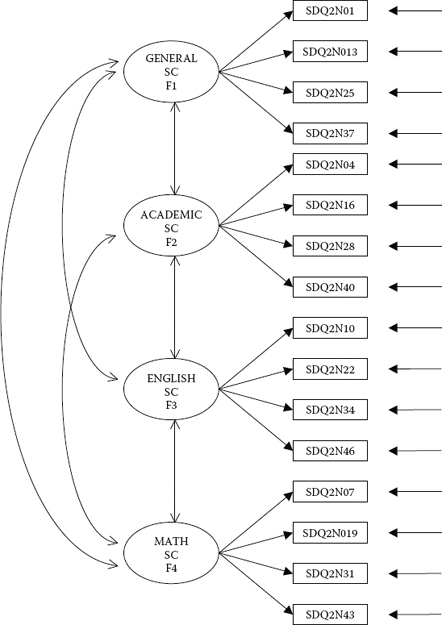
Figure 3.1. Hypothesized four-factor CFA model of self-concept.

(For a review of the literature related to these issues, see Byrne, 1996.) The task presented to us here, then, is to test the original hypothesis that SC is a four-factor structure comprising a general component (GSC), an academic component (ASC), and two subject-specific components (ESC and MSC), against two alternative hypotheses: (a) that SC is a two-factor structure comprising GSC and ASC, and (b) that SC is a one-factor structure in which there is no distinction between general and academic SCs.

We turn now to an examination and testing of each of these hypotheses.

Hypothesis 1: Self-Concept Is a Four-Factor Structure

The model to be tested in Hypothesis 1 postulates a priori that SC is a four-factor structure composed of General SC (GSC), Academic SC (ASC), English SC (ESC), and Math SC (MSC); it is presented schematically in Figure 3.1.

Before any discussion of how we might go about testing this model, let's take a few minutes first to dissect the model and list its component parts as follows:

• There are four SC factors, as indicated by the four ovals labeled General SC, Academic SC, English SC, and Math SC.
• The four factors are correlated, as indicated by the two-headed arrows.
• There are 16 observed variables, as indicated by the 16 rectangles (SDQ2N01 through SDQ2N43); they represent item pairs¹ from the General, Academic, Verbal, and Math SC subscales of the Self-Description Questionnaire II (SDQ2; Marsh, 1992).
• The observed variables load on the factors in the following pattern: SDQ2N01 to SDQ2N37 load on Factor 1, SDQ3N04 to SDQ2N40 load on Factor 2, SDQ2N10 to SDQ2N46 load on Factor 3, and SDQ2N07 to SDQ2N42 load on Factor 4.
• Each observed variable loads on one and only one factor.
• Residuals associated with each observed variable are uncorrelated.

Summarizing these observations, we can now present a more formal description of our hypothesized model. As such, we state that the CFA model presented in Figure 3.1 hypothesizes a priori that

1. SC responses can be explained by four factors: General SC, Academic SC, English SC, and Math SC;
2. each item-pair measure has a nonzero loading on the SC factor that it was designed to measure (termed a target loading) and a zero loading on all other factors (termed nontarget loadings);
3. the four SC factors, consistent with the theory, are correlated; and
4. residual errors associated with each measure are uncorrelated.

Another way of conceptualizing the hypothesized model in Figure 3.1 is within a matrix framework as presented in Table 3.1. Thinking about the model components in this format can be very helpful because it is consistent with the manner by which the results from structural equation modeling (SEM) analyses are commonly reported in program output files. The tabular representation of our model in Table 3.1 shows the pattern of parameters to be estimated within the framework of three matrices: the factor-loading matrix, the factor variance–covariance matrix, and the residual variance–covariance matrix. In statistical language, these parameter arrays are termed the lambda, psi, and theta matrices, respectively. We will revisit these matrices later in the chapter in discussion of the TECH1 Output option.

Table 3.1 Pattern of Estimated Parameters for Hypothesized Four-Factor Model

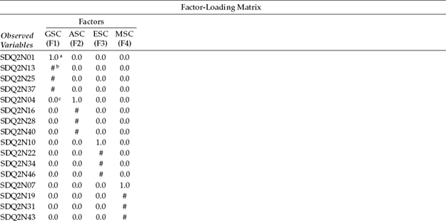
a Parameter fixed to 1.0.

b Parameter to be estimated.

c Parameter fixed to 0.0.

For purposes of model identification and latent variable scaling (see Chapter 2), you will note that the first of each congeneric set (see Chapter 2, note 2) of SC measures in the factor-loading matrix is set to 1.0, which you may recall is default in Mplus; all other parameters are freely estimated (as represented by the pound sign: #). Likewise, as indicated in the factor variance–covariance matrix, all parameters are freely estimated. Finally, in the residual variance–covariance matrix, only the residual variances are estimated; all residual covariances are presumed to be zero.

Provided with these two views of this hypothesized four-factor model, let's now move on to the testing of this model. We begin, of course, by structuring an input file that fully describes the model to Mplus.

Mplus Input File Specification and Output File Results

Input File Specification

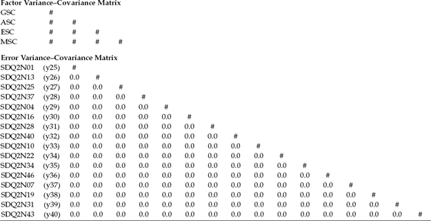
In Chapter 2, I advised you of the Mplus language generator and provided a brief description of its function and limitations, together with an illustration of how this facility can be accessed. In this first application, I now wish to illustrate how to use this valuable feature by walking you through the steps involved in structuring the input file related to Figure 3.1. Following from the language generator menu shown in Figure 2.2, we begin by clicking on the SEM option as illustrated in Figure 3.2.

Figure 3.2. Mplus language generator: Selecting category of analytic model.

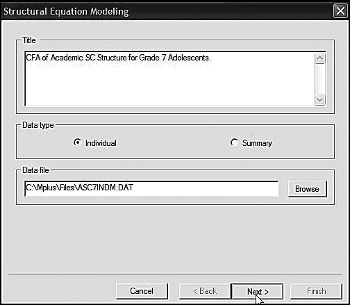
Figure 3.3. Mplus language generator: Specification of title and location of data.

Once you click on the SEM option, you will be presented with the dialog box shown in Figure 3.3. Here I have entered a title for the model to be tested (see Figure 3.1), indicated that the data represent individual scores, and provided the location of the data file on my computer. The Browse button simplifies this task.

The next dialog box presented to you (see Figure 3.4) requests information related to the data: (a) whether they are in free or fixed format and, if the latter, specifics of the Fortran statement format state; and (b) if there are any missing data. The data to be used in this application (ascindm.dat) are in fixed format as noted, and the format statement is 40F1.0, X, 6F2.0. This expression tells the program to read 40 single-digit numbers, to skip one column, and then to read six double-digit numbers. The first 40 columns represent item scores on the Self-Perception Profile for Children (SPPC; not used in the present study) and the SDQ2; the remaining six scores represent scores for the MASTENG1 through SMAT1 variables (not used in the present study). Finally, we note that there are no missing data.

The next three dialog boxes (Figures 3.5, 3.6, and 3.7) focus on the variable names. The first dialog box, shown in Figure 3.5, requests the names of all variables in the entire data set. Here you can see that they are first entered and then added to the list one at a time. In the dialog box shown in Figure 3.6, you are asked to specify which variables will actually be used in the analyses. Shown on the left side of this dialog box, you can see that I have blocked this specific set of variables, which is now ready for transfer over to the Usevariable List. Finally, Figure 3.7 shows the completion of this process.

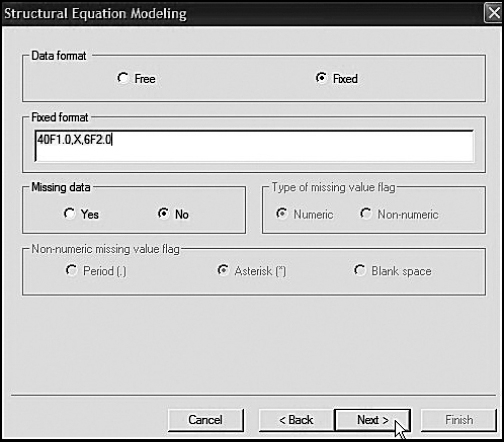
Figure 3.4. Mplus language generator: Specification of fixed format for data.

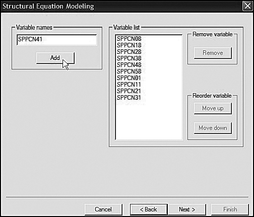
Figure 3.5. Mplus language generator: Specification and adding all observed variables in the data to the variable list.

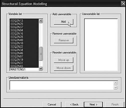
Figure 3.6. Mplus language generator: Selected observed variables to be used in the analyses.

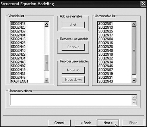
Figure 3.7. Mplus language generator: Addition of selected observed variables to the usevariable list.

The next two dialog boxes, in the present instance, do not require any additional input information; nonetheless, it is important that I show them to you in the interest of your own work in the future. The dialog box shown in Figure 3.8 provides the opportunity of specifying (a) a grouping variable, which is not applicable to the present analyses; (b) a weight variable, which is not applicable; and (c) existing categorical variables; all variables in the present data set are of continuous scale. The dialog box shown in Figure 3.9 allows for analyses based on Mean Structures or of a summative nature, as provided by the Basic option. However, it is important to note that, beginning with Mplus 5, MEANSTRUCTURE is default and the option is now NOMEANSTRUCTURE. Our analyses are categorized as the General type, which, as noted in Chapter 2, is default. Models that can be estimated in this category include regression analysis, path analysis, CFA, SEM, latent growth curve modeling, discrete-time survival analysis, and continuous-time survival analysis. Review of the middle section of this dialog box indicates that the estimator to be used in testing our hypothesized model is that of maximum likelihood (ML), which, again, is the default. Finally, the criteria for termination are automatically entered by the program, again by default.

The dialog box shown in Figure 3.10 shows the output options available to you when the language generator is used. For purposes of this first application, I have selected only three: sample statistics, modifications indices, and standardized coefficients. Of course, other additional output options can always be added to the input file after the language-generated file has been completed.

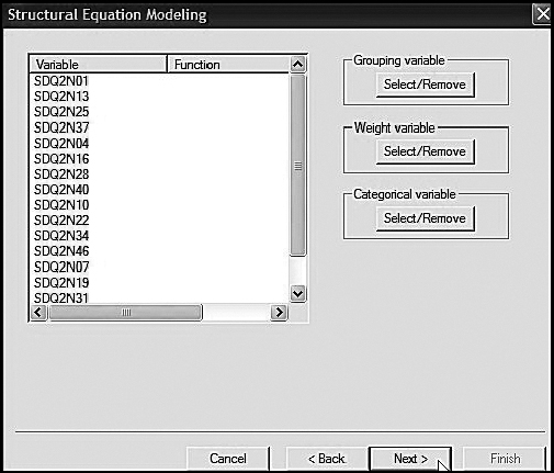
Figure 3.8. Mplus language generator: Dialog box showing additional options if needed.

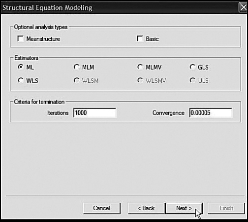
Figure 3.9. Mplus language generator: Dialog box showing default ML estimator.

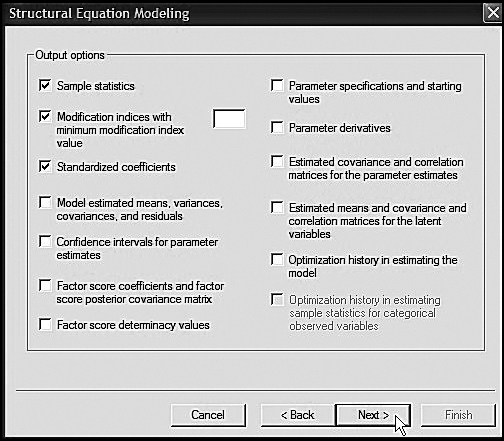
Figure 3.10. Mplus language generator: Dialog box showing selected output options.

The next two dialog boxes associated with the language generator display the final input file, albeit only a portion of it is visible in Figure 3.11 because the main dialog box includes an overlay dialog box cautioning that statements defining the MODEL and DEFINE commands must be added separately. The completed Mplus input file describing the CFA model shown in Figure 3.1 is presented in Figure 3.12. As you will note, I have added the MODEL command to the final language-generated input file. Accordingly, we see that Factor 1 (General SC) is measured by SDQ2N01 through SDQ2N37, Factor 2 (Academic SC) by SDQ2N04 through SDQ2N40, Factor 3 (English SC) by SDQ2N10 through SDQ2N46, and Factor 4 (Math SC) by SDQ2N07 through SDQ2N43. In addition, I have included the TECH1 option to the OUTPUT command as it replicates the pattern shown in Table 3.1 and, as such, can be instructive in helping you to visualize the estimated parameters within the framework of their matrices.

Now that we have finalized the input file, we are ready to execute the job and have Mplus perform the analysis. Figure 3.13 illustrates how easy this process is. Simply click on the Mplus tab, which will release the dropdown menu; then click on Run Mplus. Once the analysis is completed (typically in only a few seconds), the file is saved as an output file and is immediately superimposed on the input file; the latter is automatically saved as mptext1.inp, and the output file as mptext1.out. Of course, you can change these labels to suit your own filing preferences. Figure 3.14 illustrates both the labeling and location of these files. As you will see, I have relabeled the file as CFA.asc7F4i. As such, the input file has an “.inp extension,” whereas the output file has an “.out extension.” To retrieve these files, click on File, and in the resulting drop-down menu, click on Open. By clicking on the arrow associated with types of files, you can select either the input or output file, in addition to other files that may be listed under this particular folder (titled Chp 3 in the present case).

Output File Results

We turn now to the CFA.asc7F4i output file. Presented first in all Mplus output files is a replication of the Mplus input file. However, due to space restrictions, I have not repeated this information here (but see Figure 3.12). Initially, you might query the purpose of this duplicated information. However, this feature can be a valuable one in the event that you are presented with an error message related to your analysis, as it enables you to quickly check your specification of a model without having to switch to the original input file. I now present the remaining output material within the context of three blocks of information: “Summary of Model and Analysis Specifications,” “Model Assessment,” and “Model Misspecification.”

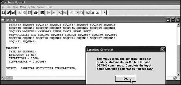
Figure 3.11. Mplus language generator: Partially completed input file showing pop-up caveat regarding MODEL and DEFINE commands.

Figure 3.12. Mplus language generator: Completed input file for hypothesized four-factor model.

Figure 3.13. Executing the Mplus input file for analysis.

Summary of Model and Analysis Specifications

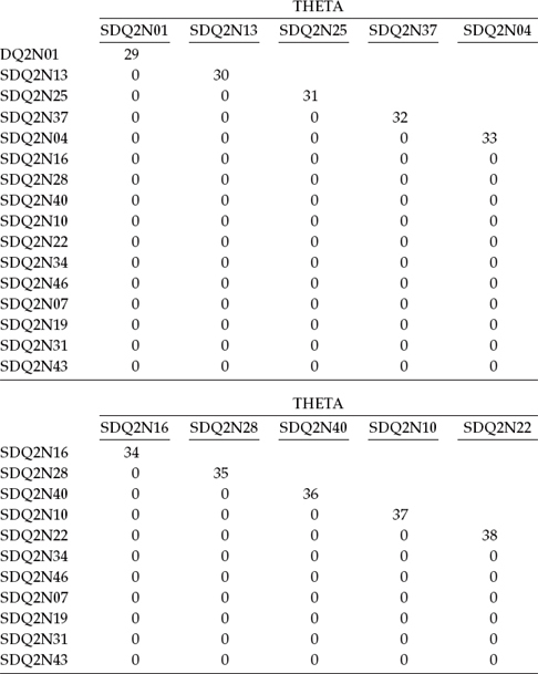
In Table 3.2, you will see a summary of model specifications related to Figure 3.1. Essentially, with exception of the first vector NU, Table 3.2 is analogous to Table 3.1 in that it details the pattern of fixed versus estimated parameters in the model. This information results from inclusion of the TECH1 option in the OUTPUT command. Accordingly, this option displays, in matrix format, all freely estimated parameters with the assignment of a numeral to each. Although this option also yields start values for each of these parameters, they are not included here in the interest of space restrictions. It is important for you to know that, under normal circumstances, the location of these TECH1 results in the output file will follow those for the modification indices. However, for my purposes in helping you to understand both the concepts of SEM and the Mplus program, I prefer to show you these arrays first as I believe they can serve importantly in helping you to formulate a mental picture of each parameter housed within its own particular matrix.

Figure 3.14. Dialog box showing selection and opening of the Mplus output file.

There are at least two important aspects of these TECH1 results that I wish to highlight for you. First, associated with each matrix and/or vector, you will observe a label bearing a Greek matrix label. These matrices and vectors are grounded in SEM theory and thus are consistently recognized across all SEM software programs. To the best of my knowledge, however, only the LISREL and Mplus programs explicitly display these parameter arrays in this manner. Indeed, knowledge of these matrices is critical in using LISREL, as its syntax is matrix based.² In Table 3.2, only one vector (NU) and three matrices (LAMBDA, THETA, and PSI) are shown as only these are relevant to the model under test in this chapter. Parameters in the NU vector represent the intercepts of continuous observed variables (in the present case, the item pair scores). The LAMBDA matrix reflects the pattern of factor loadings and, as such, is consistent with the first matrix shown in Table 3.1. In this regard, note in Table 3.2 that the first parameter of each congeneric set of observed indicator variables (e.g., SDQ2N01, SDQ2N04, SDQ2N10, and SDQ2N07) has an assigned 0 rather than a numeral, thereby indicating that it is a fixed parameter and thus is not estimated. The THETA matrix represents the residuals. As in Table 3.1, these estimated parameters appear on the outside diagonal as only estimates for the variances of these parameters are of interest; no residual covariances are specified, thus these parameters remain fixed to zero. Finally, the PSI matrix represents the variances and covariances of the continuous latent variables, in other words, the factor variances and covariances as specified in Figure 3.1.

Table 3.2 Mplus Output: Summary of Model Specifications

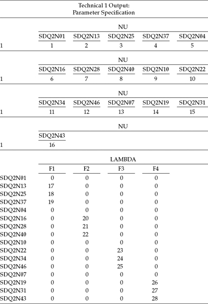
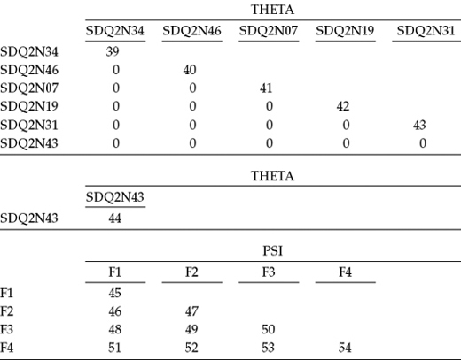
Second, the number assigned to each of the parameters shown in Table 3.2 serves three important purposes: (a) to identify, in error messages, the parameter likely to be the source of difficulty with issues related to nonidentification and other such problems; (b) to enable you to determine if all estimated parameters were specified correctly and, if not, to identify in which matrix the error occurred; and (c) to provide you with easy access to the number of parameters to be estimated. With respect to this latter point, I need to alert you to one very important aspect of the numbered parameters shown in Table 3.2. Specifically, you will note that the total number of parameters to be estimated is shown to be 54 (see the PSI matrix). However, in reviewing Figure 3.1, we see that the number of parameters to be estimated is 12 factor loadings, 16 observed variable residual variances, 4 factor variances, and 6 factor covariances, which equals 38 and not 54. Why this discrepancy? The answer lies in the fact that, by default, as discussed in Chapter 2, Mplus always includes observed variable intercepts in the model. However, if there is no structure on these parameters (i.e., they are not specified in the model), the program ignores these parameters.

Let's move on now to the next two sets of information provided in the output file. The first of these (see Table 3.3) provides a summary of the analysis specifications, and the second (see Table 3.4) reports the sample statistics as requested in the OUTPUT command, in addition to portions of both the sample covariance and correlation matrices. Turning first to Table 3.3, we see that the input file was properly structured, and, as a result, the program encountered no difficulties in reading the model specifications and other related input information. The summary information here reports the number of groups to be one and the number of cases to be 265. With respect to the model, we are advised that there are 16 dependent variables (the observed item pair scores) and 4 continuous latent variables (i.e., the factors), all of which are subsequently identified below. Finally, we note that (a) maximum likelihood was used to estimate the parameters, and (b) the name of the data file and its related input data format. The importance of this summary information is that it assures you that the program has interpreted the input instructions and read the data appropriately.

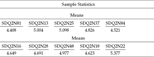
The sample statistics are reported in Table 3.4. Unfortunately, however, Mplus reports only the observed variable means (i.e., the intercepts), and not the full range of univariate and multivariate descriptive statistics when this option is requested. These values are for information only, given that these parameters are not of interest with respect to this application. Included in this table also, although in substantially abbreviated form, is a portion of the sample covariance and correlation matrices. I include this material solely to familiarize you with the structure of the Mplus output file.

Table 3.3 Mplus Output: Summary of Analysis Specifications

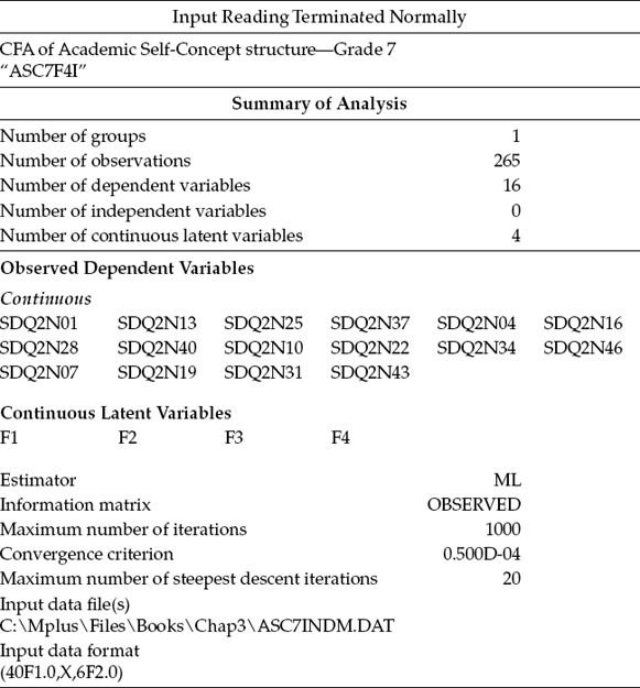
Table 3.4 Mplus Output: Sample Statistics

Assessment of Model as a Whole

Of primary interest in SEM is the extent to which a hypothesized model “fits,” or, in other words, adequately describes the sample data. Given findings of inadequate goodness-of-fit, the next logical step is to detect the source of misfit in the model. Ideally, evaluation of model fit should be based on several criteria that can assess model fit from a diversity of perspectives. In particular, these focus on the adequacy of (a) the model as a whole, and (b) the individual parameter estimates.

Before examining this section of the Mplus output, however, I consider it instructive to review four important aspects of fitting hypothesized models; these are (a) the rationale upon which the model-fitting process is based, (b) the issue of statistical significance, (c) the estimation process, and (d) the goodness-of-fit statistics.

The Model-Fitting Process

In Chapter 1, I presented a general description of this process and noted that the primary task is to determine the goodness-of-fit between the hypothesized model and the sample data. In other words, the researcher specifies a model and then uses the sample data to test the model.

With a view to helping you gain a better understanding of the material to be presented next in the output file, let's take a few moments to recast this model-fitting process within a more formalized framework. As such, let S represent the sample covariance matrix (of observed variable scores), Σ (sigma) to represent the population covariance matrix, and θ (theta) to represent a vector that comprises the model parameters. As such, Σ(θ) represents the restricted covariance matrix implied by the model (i.e., the specified structure of the hypothesized model). In SEM, the null hypothesis (H₀) being tested is that the postulated model holds in the population [i.e., Σ = Σ(θ)]. In contrast to traditional statistical procedures, however, the researcher hopes not to reject H₀ (but see MacCallum, Browne, & Sugawara, 1996, for proposed changes to this hypothesis-testing strategy).

The Issue of Statistical Significance

As you are no doubt aware, the rationale underlying the practice of statistical significance testing has generated a plethora of criticism over, at least, the past 4 decades. Indeed, Cohen (1994) has noted that, despite Rozeboom's (1960) admonition more than 50 years ago that “the statistical folkways of a more primitive past continue to dominate the local scene” (p. 417), this dubious practice still persists. (For an array of supportive as well as opposing views with respect to this article, see the American Psychologist [1995], 50, 1098–1103.) In light of this historical bank of criticism, together with the pressure by methodologists to cease this traditional ritual (see, e.g., Cohen, 1994; Kirk, 1996; Schmidt, 1996; Thompson, 1996), the Board of Scientific Affairs for the American Psychological Association (APA) appointed a task force to study the feasibility of possibly phasing out the use of null hypothesis significance (NHST) procedures, as typically described in course texts and reported in journal articles. As a consequence of findings reported and conclusions drawn by this task force (see Wilkinson and the Task Force on Statistical Inference, 1999), the APA (2010) now stresses that “NHST is but a starting point and that additional reporting elements such as effect sizes, confidence intervals, and extensive description are needed to convey the most complete meaning of results” (p. 33). (For additional perspectives on this topic, see Harlow, Mulaik, & Steiger, 1997; Jones & Tukey, 2000; Kline, 2004.)

It can be argued that NHST, with respect to the analysis of covariance structures, is somewhat different in that it is driven by degrees of freedom involving the number of elements in the sample covariance matrix and the number of parameters to be estimated. Nonetheless, it is interesting to note that many of the issues raised with respect to the traditional statistical methods (e.g., practical significance, importance of confidence intervals, and importance of replication) have long been addressed in SEM applications. Indeed, it was this very issue of practical “nonsignificance” in model testing that led Bentler and Bonett (1980) to develop one of the first subjective indices of fit (the Normed Fit Index [NFI]). Indeed, their work subsequently spawned the development of numerous additional practical indices of fit, some of which are included in the Mplus output shown in Table 3.5. Likewise, the early work of Steiger (1990; Steiger & Lind, 1980) precipitated the call for use of confidence intervals in the reporting of SEM findings (see, e.g., MacCallum et al., 1996). More recently, Rodgers (2010) has referred to this movement for change “a quiet methodological revolution.” For a comprehensive and intriguing historical review of NHST and modeling, their relation to one another, and their implications for current methodological practice, I urge you to read Rodger's very informative article, which I'm sure will become a classic in the field!

The Estimation Process

The primary focus of the estimation process, in SEM, is to yield parameter values such that the discrepancy (i.e., residual) between the sample covariance matrix S and the population covariance matrix implied by the model [Σ(θ)] is minimal. This objective is achieved by minimizing a discrepancy function, F[S, Σ(θ)], such that its minimal value (F_min) reflects the point in the estimation process where the discrepancy between S and Σ(θ) is least [S - Σ(θ) = minimum]. Taken together, then, F_min serves as a measure of the extent to which S differs from Σ(θ); any discrepancy between the two is captured by the residual covariance matrix.

Table 3.5 Mplus Output: Goodness-of-Fit Statistics

The Model Estimation Terminated Normally: Tests of Model Fit
Chi-Square Test of Model Fit
Value	159.112
Degrees of freedom	98
p-value	0.0001
Chi-Square Test of Model Fit for the Baseline Model
Value	1703.155
Degrees of freedom	120
p-value	0.0000
CFI/TLI
CFI	0.961
TLI	0.953
Loglikelihood
H0 value	-6562.678
H1 value	-6483.122
Information Criteria
Number of free parameters	54
Akaike (AIC)	13233.356
Bayesian (BIC)	13426.661
Sample-size adjusted BIC (n* = (n + 2)/24)	13255.453
Root Mean Square Error of Approximation (RMSEA)
Estimate	0.049
90% confidence interval (CI)	0.034	0.062
Probability RMSEA <= .05	0.556
Standardized Root Mean Square Residual (SRMR)
Value	0.045

The Goodness-of-Fit Statistics

Let's turn now to the model fit statistics, which are presented in Table 3.5. Here we find several goodness-of-fit values, all of which relate to the model as a whole. The first of these values represents the Chi-Square Test of Model Fit. The value of 159.112 represents the discrepancy between the unrestricted sample covariance matrix S and the restricted covariance matrix Σ(θ) and, in essence, represents the Likelihood Ratio Test statistic, most commonly expressed as a chi-square (χ²) statistic. Although this statistic is typically calculated as (N-1)F_min (sample size minus 1, multiplied by the minimum fit function), Mplus uses only a value of N, rather than N-1 (Brown, 2006). In general, H₀ Σ = Σ(θ) is equivalent to the hypothesis that Σ - Σ(θ) = 0; the χ² test, then, simultaneously tests the extent to which all residuals in Σ - Σ(θ) are zero (Bollen, 1989). Framed a little differently, the null hypothesis (H₀) postulates that specification of the factor loadings, factor variances and covariances, and residual (i.e., measurement error) variances for the model under study are valid; the likelihood ratio test statistic (χ²), then, simultaneously tests the extent to which this specification is true. The probability value associated with χ² represents the likelihood of obtaining a χ² value that exceeds the χ² value when H₀ is true. Thus, the higher the probability associated with χ², the closer the fit between the hypothesized model (under H₀) and the perfect fit (Bollen, 1989).

The test of our H₀—that SC is a four-factor structure, as depicted in Figure 3.1—yielded a χ² value of 159.112, with 98 degrees of freedom and a probability of less than .0001 (p < .0001), thereby suggesting that the fit of the data to the hypothesized model is not entirely adequate. Interpreted literally, this test statistic indicates that, given the present data, the hypothesis bearing on SC relations, as summarized in the model, represents an unlikely event (occurring less than one time in a thousand under the null hypothesis) and should be rejected. The sensitivity of the χ² likelihood ratio test to sample size, however, is well known and is addressed shortly.

The next fit statistic reported in the Mplus output is the Chi-Square Test of Model Fit for the Baseline Model, which is shown to have a χ² value of 1703.155 with 120 degrees of freedom (p < .000). Although the baseline model in most SEM computer programs represents what is commonly termed the independence (or null) model,³ the baseline model in Mplus is structured somewhat differently. Common to both baseline models is the assumption of zero covariation among the observed indicator variables. However, whereas the only parameters in the independence model related to a CFA model (such as the one in this chapter) are the observed variable variances (given that no estimated means are of interest), those in the Mplus baseline model comprise both the variances and means (i.e., intercepts) of the observed variables. As discussed earlier in this chapter in relation to Table 3.2, Mplus always estimates the observed variable intercepts even though they may not actually be part of the structured model, which is the case with the present application.

Because both baseline models assume zero covariation among the observed variables, it is not surprising that the χ² value of these models is typically always substantially larger than that of the structured hypothesized model. Indeed, this is precisely the situation here, where we find the χ² value of the hypothesized model to be 159.112 with 98 degrees of freedom versus the Mplus baseline model χ² value of 1703.155 with 120 degrees of freedom. The relevance of this comparison between the baseline and hypothesized models plays out in assessing the extent to which the hypothesized model fits the data, compared with the baseline model. To the extent that the χ² value of the hypothesized model is less than that of the baseline model, the hypothesized model is considered to exhibit an improvement of fit over the baseline model. In other words, the structured model is superior to the unstructured model.

Given the prominence of the likelihood ratio statistic (χ²) in the SEM literature, I believe it will be helpful to you if we take a slight digression before moving on to examine the remaining model fit results. As such, I hope to provide you with a framework within which to comprehend the link between the χ² statistic and other goodness-of-fit statistics reported in the SEM literature, a few of which are included in the Mplus output and discussed shortly. Specifically, I wish to alert you not only to the many problematic features of the χ² statistic but also to its more valuable uses within the model-fitting process. We turn first to the widely known difficulties associated with this statistic.

Perhaps the most challenging and frustrating aspect of the likelihood ratio test statistic is its sensitivity to sample size. Because the χ² statistic equals (N-1)F_min or (N)F_min, this value tends to be substantial when the model does not hold and the sample size is large (Jöreskog & Sörbom, 1993). The conundrum here, however, is that the analysis of covariance structures is grounded in large sample theory. As such, large samples are critical to obtaining precise parameter estimates, as well as to the tenability of asymptotic distributional approximations (MacCallum et al., 1996). Thus, findings of well-fitting hypothesized models, where the χ² value approximates the degrees of freedom, have proven to be unrealistic in most SEM empirical research. That is, despite relatively negligible difference between a sample covariance matrix (S) and its associated restricted covariance matrix (Σ), it is not unusual that a model would be rejected given a large sample size. Most common to SEM research, then, are findings of a large χ² relative to degrees of freedom, thereby indicating a need to modify the model in order to better fit the data (Jöreskog & Sörbom, 1993). Thus, results related to the test of our hypothesized model are not unexpected. Indeed, given this problematic aspect of the Likelihood Ratio Test and the fact that postulated models (no matter how good) can only ever fit real-world data approximately and never exactly, MacCallum et al. (1996) proposed changes to the traditional hypothesis-testing approach in covariance structure modeling. (For an extended discussion of these changes, see MacCallum et al., 1996.)

At least two additional problematic features of the χ² statistic are also well known. The first of these relates to conditions of small sample size and/or data that are nonnormally distributed. In such instances, the underlying distribution is not χ² distributed, thereby distorting the statistical significance of the model test (Brown, 2006). The second troublesome aspect of the χ² statistic is that it is based on the excessively stringent hypothesis that the sample covariance matrix (S) is equal to the restricted covariance matrix (Σ).

Having cautioned you about the negative aspects of the χ² statistic, allow me now to offset those rather bad features by describing two of its more notably positive ones. The first of these is the fact that the χ² statistic is used in the computation of many alternative model fit indices, most of which, if not all, were developed for the purposes of addressing particular weaknesses in the likelihood ratio test statistic as an index of model fit. (The likelihood ratio χ² statistic holds the honor of being the first index developed and used in the assessment of model fit in SEM.) Four of these alternate indices of fit are included in the Mplus output (see Table 3.5; the Comparative Fit Index [CFI], Tucker-Lewis Fit Index [TLI], Akaike's Information Criterion [AIC], and Bayes Information Criterion [BIC]) and are described shortly. The second important use of the χ² statistic is in the comparison of nested models,⁴ a mechanism used in testing for evidence of measurement and structural equivalence (i.e., invariance) across groups. These comparisons are illustrated in applications addressed in Chapters 7, 8, and 9.

Now that you are aware of both the good and not-so-good aspects of the χ² statistic, let's move on to review the remaining model fit statistics in the Mplus output in Table 3.5. As a result of the problematic features just noted regarding this statistic, you can now appreciate why researchers have been motivated to address these limitations via the development of alternative goodness-of-fit indices that take a more pragmatic approach to the evaluation process. To this end, the past 2 decades have witnessed a plethora of newly developed fit indices as well as unique approaches to the model-fitting process (for reviews, see, e.g., Gerbing & Anderson, 1993; Hu & Bentler, 1995; Marsh, Balla, & McDonald, 1988; Tanaka, 1993). In overcoming the problematic nature of the χ² statistic, a fit index quantifies the degree of model fit along a continuum (Hu & Bentler, 1999). These criteria, commonly referred to as subjective, practical, or ad hoc indices of fit, are now commonly used as adjuncts to the χ² statistic given that the latter is rarely, if ever, used as the sole index of model fit. Although the χ² statistic, by convention, is always reported, decisions regarding adequacy of model fit are typically based on alternate indices of fit, four of which we review now in Table 3.5.

In general, model fit indices fall into one of two categories: incremental (Hu & Bentler, 1995, 1999), also termed comparative (Browne, MacCallum, Kim, Andersen, & Glaser, 2002), and absolute, with incremental indices seemingly being the most widely used in SEM. Whereas incremental indices of fit measure the proportionate improvement in fit of a hypothesized model compared with a more restricted, albeit nested, baseline model (Hu & Bentler, 1999), absolute indices of fit assess the extent to which an a priori model reproduces the sample data. That is, in contrast to incremental fit indices, no reference model is used in determining the amount of improvement in model fit. Nonetheless, either an implicit or explicit comparison may be made to a saturated model⁵ that exactly reproduces the sample covariance matrix (Hu & Bentler, 1999).

More recently, there has been a tendency to consider a third category of fit indices sometimes referred to as predictive indices of fit (e.g., Kline, 2011) and other times as parsimony-corrective indices of fit (e.g., Brown, 2006). This third category, however, is much less clearly defined than the two primary fit index categories, as a review of the SEM literature reveals not only an overlapping of these characteristics (predictability and parsimony correction) but also the tendency on the part of some authors to categorize them as either incremental or absolute indices of fit. Thus, in describing the goodness-of-fit statistics reported in the Mplus output reported in Table 3.5, I include this third category but refer to it as the predictive or parsimony-corrected category. Characteristics of this rather tenuous category are presented later in conjunction with details of its two related fit indices, the AIC and BIC. We turn now to a description of all model indices of fit.

Two of the most commonly used incremental indices of fit in SEM are the CFI (Bentler, 1990) and the TLI (Tucker & Lewis, 1973). Both measure the proportionate improvement in model fit by comparing the hypothesized model in which structure is imposed with the less restricted nested baseline model. Values for the CFI are normed in the sense that they range from zero to 1.00, with values close to 1.00 being indicative of a well-fitting model. Although a value > .90 was originally considered representative of a well-fitting model (see Bentler, 1992), a revised cutoff value close to .95 has more recently been advised (Hu & Bentler, 1999). Computation of the CFI is as follows:

where H = the hypothesized model, and B = the baseline model.

Based on the results reported in Table 3.5, this equation translates into

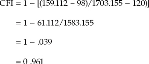
This value, of course, is consistent with the CFI value of 0.961 reported in Table 3.5 and assures us that the hypothesized four-factor model displayed in Figure 3.1 fits our sample of Grade 7 adolescents very well.

In contrast to the CFI, the TLI is a nonnormed index, which means that its values can extend outside the range of 0.0 to 1.0. This condition explains why some computer programs refer to the TLI as the non-normed index. This feature of the TLI notwithstanding, it is customary to interpret its values in the same way as for the CFI, with values close to 1.0 being indicative of a well-fitting model. A second differentiating aspect of the TLI, compared with the CFI, is its inclusion of a penalty function for models that are overly complex. What I mean by this statement is that when a model under study includes parameters that contribute minimally to improvement in model fit, this fact is taken into account in the computation of the TLI value. Computation of the TLI is as follows:

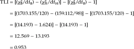
As reported in Table 3.5, we see that this value replicates the reported TLI value of 0.953, and is consistent with that of the CFI in advising that our hypothesized four-factor SC model is very well-fitting, thereby describing the sample data extremely well.

Turning again to the Mplus output in Table 3.5, I draw your attention now to the next two sets of information provided. The first set, listed under the heading Loglikelihood, reports two loglikelihood values—one for the hypothesized model (H₀ value) and one for the baseline model (H₁ value). These values are used in computation of the two model fit indices listed under the second heading, “Information Criteria.”

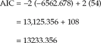
We turn now to the second heading and these two model fit indices, the AIC (Akaike, 1987) and BIC (Raftery, 1993; Schwartz, 1978), both of which are considered candidates for the predictive and parsimony-corrected category of fit indices. In contrast to the CFI and TLI, both of which focus on comparison of nested models, the AIC and BIC are used in the comparison of two or more nonnested models, with the smallest value overall representing the best fit of the hypothesized model. Both the AIC and BIC take into account model fit (as per the χ² value) as well as the complexity of the model (as per model degrees of freedom or number of estimated parameters). The BIC, however, assigns a greater penalty in this regard and, thus, is more apt to select parsimonious models (Arbuckle, 2007).

Of these two indices, the AIC is the more commonly used in SEM. This is particularly so with respect to the situation where a researcher proposes a series of plausible models and wishes to determine which one in the series yields the best fit (Raykov & Marcoulides, 2000), as well as reflects the extent to which parameter estimates from an original sample will cross-validate in future samples (Bandalos, 1993). In this latter sense, the AIC is akin to the Expected Cross-Validation Index (ECVI; Browne & Cudeck, 1989), another popular index included in most computer SEM packages, although not in the Mplus program. Given the similar application of the AIC and BIC, albeit the more common usage of the former, an example calculation of only the AIC is presented here.

Interestingly, at least three versions of computation exist with respect to the AIC with the result that these versions vary across SEM computer software (Brown, 2006). These differences notwithstanding, they have been shown to be equivalent (see Kaplan, 2000). Computation of the AIC pertinent to the Mplus program is as follows:

where loglikelihood refers to the H₀ value and a is the number of estimated parameters. Recall that Mplus always computes estimates for the observed variable intercepts, regardless of whether or not they are structured in the model. Thus, although the actual number of estimated parameters in our hypothesized four-factor model is 38, Mplus considers the number of estimated parameters here to be 54 (38 + 16 intercepts).

The last two model fit indices listed in Table 3.5, the Root Mean Square Error of Approximation (RMSEA; Steiger & Lind, 1980) and the Standardized Root Mean Square Residual (SRMR), belong to the category of absolute indices of fit. However, Browne and colleagues (2002) have termed them, more specifically, as “absolute misfit indices” (p. 405). In contrast to incremental fit indices, as noted earlier, absolute fit indices do not rely on comparison with a reference model in determining the extent of model improvement; rather, they depend only on determining how well the hypothesized model fits the sample data. Thus, whereas incremental fit indices increase as goodness-of-fit improves, absolute fit indices decrease as goodness-of-fit improves, thereby attaining their lower-bound values of zero when the model fits perfectly (Browne et al., 2002).

The RMSEA and the conceptual framework within which it is embedded were first proposed by Steiger and Lind in 1980, yet failed to gain recognition until approximately 1 decade later, as one of the most informative criteria in covariance structure modeling. The RMSEA takes into account the error of approximation in the population and asks the question “How well would the model, with unknown but optimally chosen parameter values, fit the population covariance matrix if it were available?” (Browne & Cudeck, 1993, pp. 137–138). This discrepancy, as measured by the RMSEA, is expressed per degree of freedom, thus making it sensitive to the number of estimated parameters in the model (i.e., the complexity of the model); values less than .05 indicate good fit, and values as high as .08 represent reasonable errors of approximation in the population (Browne & Cudeck, 1993). MacCallum et al. (1996), in elaborating on these cutpoints, noted that RMSEA values ranging from .08 to .10 indicate mediocre fit, and those greater than .10 indicate poor fit. Although Hu and Bentler (1999) have suggested a value of .06 to be indicative of good fit between the hypothesized model and the observed data, they cautioned that when the sample size is small, the RMSEA tends to overreject true population models. Noting that these criteria are based solely on subjective judgment, and therefore cannot be regarded as infallible or correct, Browne and Cudeck (1993) and MacCallum et al. (1996) nonetheless argued that they would appear to be more realistic than a requirement of exact fit, where RMSEA = 0.0. (For a generalization of the RMSEA to multiple independent samples, see Steiger, 1998.)

Overall, MacCallum and Austin (2000) have strongly recommended routine use of the RMSEA for at least three reasons: (a) It would appear to be adequately sensitive to model misspecification (Hu & Bentler, 1998), (b) commonly used interpretative guidelines would appear to yield appropriate conclusions regarding model quality (Hu & Bentler, 1998, 1999), and (c) it is possible to build confidence intervals around RMSEA values.

Now, let's examine computation of the RMSEA, which involves a two-step process. This index approximates a noncentral χ² distribution, which does not require a true null hypothesis; that is to say, it assumes that the hypothesized model is somewhat imperfect. In contrast to the usual χ² distribution, the noncentral χ² distribution has an additional parameter termed the noncentrality parameter (NCP), which is typically assigned the lowercase Greek symbol of delta (δ). The function of δ is to measure the extent to which the specified model (i.e., the null hypothesis) is false. Thus, as the hypothesized model becomes increasingly false, the value of δ becomes greater.

In essence, then, δ can be considered a gauge of the extent to which the hypothesized model is misspecified in one of two ways: (a) Its estimated value (δ_H) represents the difference between the hypothesized model (χ²_H) and its related number of degrees of freedom (df_H), or (b) its difference from zero in the event that the value for δ_H is negative (which is not permissible). Measuring discrepancy in fit (represented by δ) per each degree of freedom in the model therefore makes it possible for the RMSEA to compensate for the effect of model complexity. In summary, the greater the model complexity, the larger the δ value and, ultimately, the larger the RMSEA value. Expressed in equation form, the estimation of δ_H is as follows:

where max represents either (χ²_H – df_H) or zero, whichever is greater.

In contrast to χ², which measures the extent to which a hypothesized model fits exactly in the population, the RMSEA assesses the extent to which it fits reasonably well in the population. For this reason, then, it is considered an “error of approximation” index (Brown, 2006). In computation of the RMSEA, this distinction between the central and noncentral χ² values is taken into account, and the δ_H value is generally rescaled as follows:

Importantly, however, this rescaling process can vary slightly across SEM computer programs. Mplus, for example, adjusts the equation as follows:

The resulting computation of the RMSEA, based on the Mplus δ_H formula, is as follows:

Applying the two-step RMSEA formula to our own model tested in this application yields the following result:

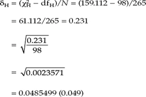
As you can see, this result is consistent with the value as shown in Table 3.5 in reflecting that our hypothesized CFA model is sufficiently parsimonious and well fitting.

Addressing Steiger's (1990) call for the use of confidence intervals to assess the precision of RMSEA estimates, Mplus reports a 90% interval around the RMSEA value. In contrast to point estimates of model fit (which do not reflect the imprecision of the estimate), confidence intervals can yield this information, thereby providing the researcher with more assistance in the evaluation of model fit. Thus, MacCallum et al. (1996) strongly urged the use of confidence intervals in practice. Presented with a small RMSEA, albeit a wide confidence interval, a researcher would conclude that the estimated discrepancy value is quite imprecise, thereby negating any possibility to determine accurately the degree of fit in the population. In contrast, a very narrow confidence interval would argue for good precision of the RMSEA value in reflecting model fit in the population (MacCallum et al., 1996).

Turning to Table 3.5, we see that our RMSEA value of .049 has a 90% confidence interval ranging from .034 to .062. Interpretation of the confidence interval indicates that we can be 90% confident that the true RMSEA value in the population will fall within the bounds of .034 and .062, which represents a good degree of precision. Given that (a) the RMSEA point estimate is < .05 (.049), and (b) the upper bound of the 90% interval is .062, which is less than the value suggested by Browne and Cudeck (1993), albeit equal to the cutoff value proposed by Hu and Bentler (1999), we can conclude that the initially hypothesized model fits the data well enough.

Before leaving this discussion of the RMSEA, it is important to note that confidence intervals can be influenced seriously by sample size as well as model complexity (MacCallum et al., 1996). For example, if sample size is small and the number of estimated parameters large, the confidence interval will be wide. Given a complex model (i.e., a large number of estimated parameters), a very large sample size would be required in order to obtain a reasonably narrow confidence interval. On the other hand, if the number of parameters is small, then the probability of obtaining a narrow confidence interval is high, even for samples of rather moderate size (MacCallum et al., 1996).

The Root Mean Square Residual (RMR) represents the average residual value derived from the fitting of the variance–covariance matrix for the hypothesized model Σ(θ) to the variance–covariance matrix of the sample data (S). However, because these residuals are relative to the sizes of the observed variances and covariances, they are difficult to interpret. Thus, they are best interpreted in the metric of the correlation matrix (Hu & Bentler, 1995; Jöreskog & Sörbom, 1989), which is represented by its standardized value (the SRMR). The SRMR represents the average value across all standardized residuals, and ranges from zero to 1.00; in a well-fitting model, this value will be small (say, .05 or less). In reviewing the output in Table 3.5, we see that the SRMR value is .045. Given that the SRMR represents the average discrepancy between the observed sample and hypothesized correlation matrices, we can interpret this value as meaning that the model explains the correlations to within an average error of .045.

Having worked your way through these goodness-of-fit measures and their computation, you may be wondering what you do with all this information. Although you certainly don't need to report the entire set of fit indices as reported in Table 3.5, such information, nonetheless, can give you a good sense of how well your model fits the sample data. But, how does one choose which indices are appropriate in the assessment of model fit? Unfortunately, this choice is not a simple one, largely because particular indices have been shown to operate somewhat differently given the sample size, estimation procedure, model complexity, and/or violation of the underlying assumptions of multivariate normality and variable independence (Fan & Sivo, 2007; Saris, Satorra, & van der Veld, 2009). Thus, in choosing which goodness-of-fit indices to use in the assessment of model fit, careful consideration of these critical factors is essential, and the use of multiple, albeit complementary, indices is highly recommended (Fan & Sivo, 2005; Hu & Bentler, 1995). In reporting results for the remaining applications in this volume, goodness-of-fit indices will be limited to the CFI, TLI, RMSEA, and SRMR, along with the related χ² value and RMSEA 90% confidence interval. Readers interested in acquiring further elaboration on the above goodness-of-fit statistics, in addition to many other indices of fit, their formulae and functions, and/or the extent to which they are affected by sample size, estimation procedures, misspecification, and/or violations of assumptions, are referred to Bandalos (1993); Bentler and Yuan (1999); Bollen (1989); Browne and Cudeck (1993); Curran, West, and Finch (1996); Fan, Thompson, and Wang (1999); Finch, West, and MacKinnon (1997); Gerbing and Anderson (1993); Hu and Bentler (1995, 1998, 1999); Hu, Bentler, and Kano (1992); Jöreskog and Sörbom (1993); La Du and Tanaka (1989); Marsh et al. (1988); Mulaik et al. (1989); Raykov and Widaman (1995); Sugawara and MacCallum (1993); Tomarken and Waller (2005); Weng and Cheng (1997); West, Finch, and Curran (1995); Wheaton (1987); and Williams and Holahan (1994); for an annotated bibliography, see Austin and Calderón (1996).

In finalizing this section on model assessment, I wish to leave you with this important reminder—that global fit indices alone cannot possibly envelop all that needs to be known about a model in order to judge the adequacy of its fit to the sample data. As Sobel and Bohrnstedt (1985) so cogently stated over 2 decades ago, “Scientific progress could be impeded if fit coefficients (even appropriate ones) are used as the primary criterion for judging the adequacy of a model” (p. 158). They further posited that, despite the problematic nature of the χ² statistic, exclusive reliance on goodness-of-fit indices is unacceptable and, indeed, provides no guarantee whatsoever that a model is useful. In fact, it is entirely possible for a model to fit well and yet still be incorrectly specified (Wheaton, 1987). (For an excellent review of ways by which such a seemingly dichotomous event can happen, readers are referred to Bentler and Chou, 1987.) Fit indices yield information bearing only on the model's lack of fit. More importantly, they can in no way reflect the extent to which the model is plausible; this judgement rests squarely on the shoulders of the researcher. Indeed, Saris et al. (2009) have recently questioned the validity of goodness-of-fit indices in the evaluation of model fit given that they are incapable of providing any indication of the “size” of a model's misspecification. Thus, assessment of model adequacy must be based on multiple criteria that take into account theoretical, statistical, and practical considerations.

Assessment of Individual Parameter Estimates

Thus far in our discussion of model fit assessment, we have concentrated on the model as a whole. Now, we turn our attention to the fit of individual parameters in the model. There are two aspects of concern here: (a) the appropriateness of the estimates, and (b) their statistical significance.

Feasibility of Parameter Estimates

The initial step in assessing the fit of individual parameters in a model is to determine the viability of their estimated values. In particular, parameter estimates should exhibit the correct sign and size, and be consistent with the underlying theory. Any estimates falling outside the admissible range signal a clear indication that either the model is wrong or the input matrix lacks sufficient information. Parameter estimates taken from covariance or correlation matrices that are not positive definite, as well as estimates exhibiting out-of-range values such as correlations > 1.00 and negative variances (known as Heywood cases), exemplify unacceptable estimated values.

Appropriateness of Standard Errors

Another indicator of poor model fit is the presence of standard errors that are excessively large or small. For example, if a standard error approaches zero, the test statistic for its related parameter cannot be defined (Bentler, 2005). Likewise, standard errors that are extremely large indicate parameters that cannot be determined (Jöreskog & Sörbom, 1989). Because standard errors are influenced by the units of measurement in observed and/ or latent variables, as well as the magnitude of the parameter estimate itself, no definitive criteria of “small” and “large” have been established (see Jöreskog & Sörbom, 1989).

Statistical Significance of Parameter Estimates

The test statistic here represents the parameter estimate divided by its standard error; as such, it operates as a z-statistic in testing that the estimate is statistically different from zero. Based on an α level of .05, then, the test statistic needs to be > ±1.96 before the hypothesis (that the estimate = 0.0) can be rejected. Nonsignificant parameters, with the exception of error variances, can be considered unimportant to the model; in the interest of scientific parsimony, albeit given an adequate sample size, they should be deleted from the model. On the other hand, it is important to note that nonsignificant parameters can be indicative of a sample size that is too small (K. G. Jöreskog, personal communication, January 1997).

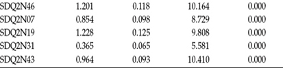
Let's turn now to this part of the Mplus output, as presented in Table 3.6. Scanning the output, you will see five columns of information, with the first column on the left listing the names of the parameters, grouped according to their model function. The initial four blocks of parameters headed with the word BY (e.g., F1------BY) represent the factor loadings. The next three blocks, headed with the word WITH (F2 WITH F1), represent the factor covariances. Finally, the last three blocks of parameters represent, respectively, the observed variable intercepts, the factor variances, and the residual variances associated with the observed variables. All estimate information is presented in the remaining four columns, with unstandardized parameter estimates presented in Column 2, standard errors in Column 3, z-scores (i.e., an estimate divided by its standard error) in Column 4, and the two-tailed probability associated with these parameter estimates appearing in Column 5.

Table 3.6 Mplus Output: Unstandardized Parameter Estimates

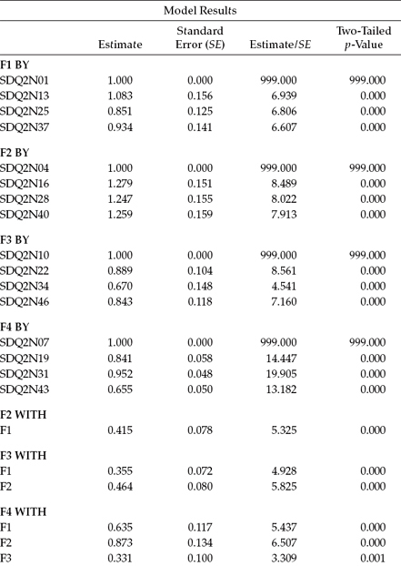
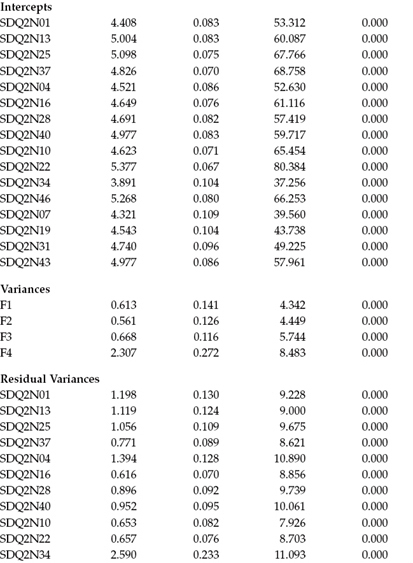
Turning to the unstandardized estimates reported in Table 3.6, let's look first at only the factor loadings. Here we note that for variables SDQ2N01, SDQ2N04, SDQ2N10, and SDQ2N07, the estimates all have a value of 1.00; their standard errors, a value of 0.00; and their z-values and probabilities, a value of 999.00. These values, of course, were fixed to 1.00 for purposes of identification and, thus, not freely estimated. All remaining factor-loading parameters, however, were freely estimated. A review of this information reveals all estimates to be reasonable (Column 2), as well as statistically significant as indicated by values > 1.96 (Column 4), and all standard errors (Column 3) to be in good order.

In contrast to other SEM programs, Mplus does not provide standardized estimates by default. Thus, if these estimates are of interest, the STANDARDIZED option must be added to the OUTPUT command statement. Once added, three types of standardization are provided by default, together with R-SQUARED values for both the observed and latent dependent variables in the model. Note, however, that users can opt for results based on only one of these three types of standardization as follows:

• STDYX: Standardization is based on background and outcome variables.
• SDY: Standardization is based on variances of continuous latent variables (i.e., factors), as well as variances of background and outcome variables.
• STD is based on variances of the continuous latent variables (i.e., factors).

Now that you are aware of the three types of standardization available in Mplus, no doubt you are wondering (as I did) which one is the correct one to use. However, it is not a matter of one being correct and the others not. It's just that there are many ways of conceptualizing standardization (L. Muthén, personal communication, February 20, 2010). As a result, SEM programs can vary in the manner by which they standardize estimates. For example, whereas the EQS program (Bentler, 2005) uses all variables in the linear structural equation system, including measurement and residual (i.e., disturbance) variances (Bentler, 2005), the LISREL program (Jöreskog & Sörbom, 1996) uses neither the measured variables nor their error and residual terms in the standardization process (see Byrne, 2006, p. 108, note 12). In contrast, Mplus provides users with the opportunity to choose their method of choice.

In the current application, estimates were based on the STDYX standardization; they are reported in Table 3.7. In reviewing these estimates, you will want to verify that particular parameter values are consistent with the literature. For example, within the context of the present application, it is of interest to inspect correlations among the SC factors in seeking evidence of their consistency with previously reported values; in the present example, these estimates met this criterion.

In addition, there are two other aspects of standardized estimates that are worthy of mention. First, note that parameters reported as 1.0 in the unstandardized solution (SDQ2N01, SDQ2N04, SDQ2N10, and SDQ2N07) take on new values in the standardized solution. Second, note also that all factor variances are reported as 1.00 with the consequence that no other information is reported for these parameters. These values remain the same regardless of which standardization is used, as in standardized solutions all variables are rescaled to have a variance of 1.00.

In closing out this section on standardized estimates, we return to the R² values mentioned earlier. Whenever the standardized estimates are requested in the OUTPUT command, an R² value and its standard error are reported for each observed and latent dependent variable in the model. Each R² value reported in Table 3.8 represents the proportion of variance in each observed variable accounted for by its related factor; it is computed by subtracting the square of the residual (i.e., measurement error) term from 1.0. (In factor analytic terms, these R² values are termed communalities.) In reviewing these values in Table 3.8, we can see that the observed variable, SDQ2N34 measuring English SC (see Figure 3.1) and having an R² of .104, appears to be the weakest of the indicator variables.

Model Misspecification

Determination of misspecified parameters is accomplished in Mplus by means of the Modification Index (MI) proposed by Sörbom (1989) for the case where all y variables are continuous and multivariate normal.⁶ Essentially, the function of the MI is to identify parameter constraints that are badly chosen. As such, all fixed parameters (i.e., those fixed to a value of 0.00) and/or those constrained to the value of another parameter (not the case in the present application) are assessed to identify which parameters, if freely estimated, would contribute to a significant drop in the χ² statistic. Results for our hypothesized model are presented in Table 3.9.

Table 3.7 Mplus Output: Standardized Parameter Estimates

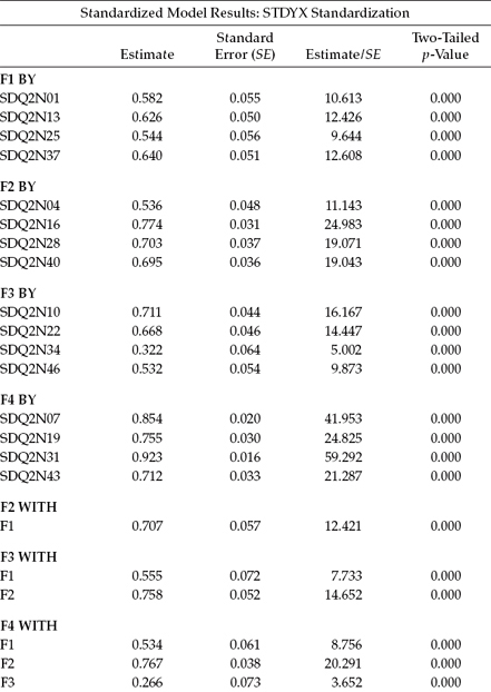
Table 3.8 Mplus Output: R-SQUARE Values for Observed Variables

Table 3.9 Mplus Output:Modification Indices (MIs)

Note: Modification indices for direct effects of observed dependent variables regressed on covariates may not be included. To include these, request MODINDICES (ALL). Minimum MI value for printing the modification index 10.000.

In reviewing these results, you will note that they appear in five columns, with the names of the variables appearing in the first column on the left, followed by their related analytic information in the remaining four columns. The MI value appears in Column 2 and represents the approximate amount by which the χ² value would decrease if the cited parameter were to be specified and freely estimated in a subsequent model. Presented in Column 3 are results for the expected parameter change (EPC) statistic (Saris, Satorra, & Sörbom, 1987). This statistic represents the predicted estimated change in either a positive or negative direction for each fixed parameter in the model should it be estimated in a subsequent test of the model. Finally, the last two columns represent two standardized versions of the EPC statistics; the STD EPC and the STDYX EPC.

Reviewing the results in Table 3.9, we see only four variables identified by Mplus as representing possibly misfitting parameters in the model. In other words, this information suggests that if these parameters were freely estimated, their specification would lead to a better fitting model. By default, as noted in the output file, Mplus reports only those parameters having an MI value equal to or greater than 10.00.⁷ Given this default, we see only four parameters specified in Table 3.9—one factor loading, as is evident from the BY statement (F2 BY SDQ2N07), and three covariances, as indicated by the WITH statements.

Let's now inspect these four parameters a little more closely. We turn first to the factor loading (F2 BY SDQ2N07). This MI represents a secondary factor loading (also termed a cross-loading), suggesting that if the observed variable SDQ2N07 (designed to measure Math SC; Factor 4) were to load additionally onto Factor 2 (Academic SC), the overall model χ² value would decrease by approximately 11.251 and this parameter's unstandardized estimate would be approximately -0.563. Although the EPC can be helpful in determining whether a parameter identified by the MI is justified as a candidate for respecification as a freely estimated parameter, Bentler (2005) has cautioned that these EPC statistics are sensitive to the way by which variables and factors are scaled or identified. Thus, their absolute values can sometimes be difficult. In the present case, from a substantive perspective, I would definitely be concerned that the EPC value is negative (-0.563), as any relation between SDQ2N07 and Academic SC should be positive.

Turning to information related to the three remaining MIs, we see that they all represent covariances between specified observed variables. However, given that (a) the observed variables in a CFA model are always dependent variables in the model, and (b) in SEM neither variances nor covariances of dependent variables are eligible for estimation, these MIs must necessarily represent observed variable residual covariances. Accordingly, these MI results suggest that if we were to estimate, for example, a covariance between the residuals associated with SDQ2N25 and SDQ2N01, the approximate value of this estimated residual covariance would be 0.359.

Overall, both the MIs and their related EPCs, although admittedly > 10.00, are very small and not worthy of inclusion in a subsequently specified model. Of prime importance in determining whether or not to include additional parameters in the model is the extent to which (a) they are substantively meaningful, (b) the existing model exhibits adequate fit, and (c) the EPC value is substantial. Superimposed on this decision is the ever constant need for scientific parsimony. Because model respecification is commonly conducted in SEM in general, as well as in several applications highlighted in this book, I consider it important to provide you with a brief overview of the various issues related to these post hoc analyses.

Post Hoc Analyses

In the application of SEM in testing for the validity of hypothesized models, the researcher will be faced, at some point, with the decision of whether or not to respecify and reestimate the model. If he or she elects to follow this route, it is important to realize that analyses will then be framed within an exploratory rather than a confirmatory mode. In other words, once a hypothesized CFA model has been rejected, this spells the end of the confirmatory factor analytic approach in its truest sense. Although CFA procedures continue to be used in any respecification and reestimation of the model, these analyses are exploratory in the sense that they focus on the detection of misfitting parameters in the originally hypothesized model. Such post hoc analyses are conventionally termed specification searches (see MacCallum, 1986). (The issue of post hoc model fitting is addressed further in Chapter 9 in the section dealing with cross-validation.)

The ultimate decision underscoring whether or not to proceed with a specification search is threefold, and focuses on substantive as well as statistical aspects of the MI results. First, the researcher must determine whether the estimation of the targeted parameter is substantively meaningful. If, indeed, it makes no sound substantive sense to free up the parameter exhibiting the MI value, one may wish to consider the parameter having the next largest value (Jöreskog, 1993). Second, both the MI and EPC values should be substantially large. Third, one needs to consider whether or not the respecified model would lead to an overfitted model. The issue here is tied to the idea of knowing when to stop fitting the model, or, as Wheaton (1987) phrased the problem, “knowing … how much fit is enough without being too much fit” (p. 123). In general, over-fitting a model involves the specification of additional parameters in the model after having determined a criterion that reflects a minimally adequate fit. For example, an overfitted model can result from the inclusion of additional parameters that (a) are “fragile” in the sense of representing weak effects that are not likely replicable; (b) lead to a significant inflation of standard errors; and (c) influence primary parameters in the model, even though their own substantive meaningfulness is somewhat equivocal (Wheaton, 1987). Although residual covariances often fall into this latter category,⁸ there are many situations, particularly with respect to social psychological research, where these parameters can make strong substantive sense and therefore should be included in the model (Cole, Ciesla, & Steiger, 2007; Jöreskog & Sörbom, 1993).

Having laboriously worked our way through the process involved in testing for the validity of this initial postulated model, what can we conclude regarding the CFA model under scrutiny in this chapter? In answering this question, we must necessarily pool all the information gleaned from our study of the Mplus output. Taking into account (a) the feasibility and statistical significance of all parameter estimates; (b) the substantially good fit of the model, with particular reference to the CFI (.961) and RMSEA (.049) values; and (c) the lack of any substantial evidence of model misfit, I conclude that any further incorporation of parameters into the model would result in an overfitted model. Indeed, MacCallum, Roznowski, and Necowitz (1992) have cautioned that “when an initial model fits well, it is probably unwise to modify it to achieve even better fit because modifications may simply be fitting small idiosyncratic characteristics of the sample” (p. 501). Adhering to this caveat, I conclude that the four-factor model schematically portrayed in Figure 3.1 represents an adequate description of self-concept structure for Grade 7 adolescents.

In keeping with the goals of the original study (Byrne & Worth Gavin, 1996), we turn next to the first alternative hypothesis—that SC for Grade 7 adolescents is a two-factor model consisting of only the constructs of General SC and Academic SC.

Hypothesis 2: Self-Concept Is a Two-Factor Structure

The model to be tested here postulates a priori that SC is a two-factor structure consisting of GSC and ASC. As such, it argues against the viability of subject-specific academic SC factors. As with the four-factor model, the four GSC measures load onto the GSC factor; in contrast, all other measures load onto the ASC factor. This hypothesized model is represented schematically in Figure 3.15, and the Mplus input file is shown in Figure 3.16.

Mplus Input File Specification and Output File Results

Input File

In reviewing these graphical and equation model specifications, three points relative to the modification of the input file are of interest. First, although the pattern of factor loadings remains the same for the GSC and ASC measures, it changes for both the ESC and MSC measures in allowing them to load onto the ASC factor. Second, because only one of these 12 ASC factor loadings needs to be fixed to 1.0, the two previously constrained parameters (SDQ2N10 and SDQ2N07) are now freely estimated. Finally, given that the observed variables specified in this analysis are sequentially listed in the data file, we need to enter only two rows of specifications under the MODEL command in the Mplus input file.

Output File

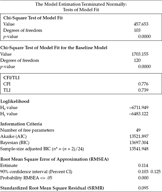
Because only the goodness-of-fit statistics are relevant to the present application, these sole results are presented in Table 3.10. In reviewing this output file, I limit our examination to only the χ² statistic and the CFI, TLI, and RMSEA indices, which are shown as framed within the rectangular boxes. As indicated here, the χ²(₁₀₃) value of 457.653 clearly represents a poor fit to the data, and certainly a substantial decrement from the overall fit of the four-factor model (χ²_[98] = 159.112). The gain of five degrees of freedom can be explained by the estimation of two fewer factor variances and five fewer factor covariances, albeit the estimation of two additional factor loadings (formerly SDQ2N10 and SDQ2N07). As expected, all other indices of fit reflect the fact that SC structure is not well represented by the hypothesized two-factor model. In particular, the CFI value of .776, TLI value of .739, and RMSEA value of .114 are strongly indicative of inferior goodness-of-fit between the hypothesized two-factor model and the sample data.

Figure 3.15. Hypothesized two-factor CFA model of self-concept.

Figure 3.16. Mplus language generator: Input file for hypothesized two-factor model.

Finally, we turn to our third and last alternative model, which postulates that adolescent SC is a unidimensional, rather than a multidimensional, construct.

Hypothesis 3: Self-Concept Is a One-Factor Structure

Although it now seems obvious that a multidimensional model best represents the structure of SC for Grade 7 adolescents, there are still researchers who contend that self-concept is a unidimensional construct. Thus, for purposes of completeness, and to address the issue of unidimensionality, Byrne and Worth Gavin (1996) proceeded in testing the above hypothesis. However, because the one-factor model represents a restricted version of the two-factor model, and thus cannot possibly represent a better fitting model, in the interest of space, these analyses are not presented here.

Table 3.10 Mplus Output: Goodness-of-Fit Statistics for Two-Factor Model

In summary, it is evident from these analyses that both the two-factor and one-factor models of SC represent a misspecification of factorial structure for early adolescents. Based on these findings, then, Byrne and Worth Gavin (1996) concluded that SC is a multidimensional construct, which in their study comprised the four facets of general, academic, English, and mathematics SCs.

Notes

1.	The use of item pairs is consistent with other construct validity research based on the Self-Description Questionnaire (SDQ) instruments conducted by Marsh and colleagues (see Byrne, 1996; Marsh, 1992).
2.	LISREL (see Jöreskog & van Thillo, 1972) is considered to be the first SEM computer program produced. Although Wolfle (2003) noted that for all practical purposes, this 1972 article described LISREL I, in actuality the first commercially produced LISREL program was marketed as LISREL III (see Byrne, in press; Sörbom, 2001).
3.	The independence (or null) model is so named as it represents complete independence of all variables in the model (i.e., all variables in the model are mutually uncorrelated). Beginning with the work of Tucker and Lewis (1973), the independence baseline model appears to be the one most widely used (Rigdon, 1996).
4.	Nested models are hierarchically related to one another in the sense that their parameter sets are subsets of one another (i.e., particular parameters are freely estimated in one model but fixed to zero in a second model) (Bentler & Chou, 1987; Bollen, 1989).
5.	A saturated model is one in which the number of estimated parameters equals the number of data points (i.e., variances and covariances of the observed variables), as in the case of the just-identified model discussed in Chapter 2. In contrast to the baseline (or independence) model, which is the most restrictive SEM model, the saturated model is the least restricted SEM model. Conceptualized within the framework of a continuum, the saturated (i.e., least restricted) model would represent one extreme endpoint, whereas the independence (the most restricted) model would represent the other; a hypothesized model will always represent a point somewhere between the two.
6.	For details regarding the formulation of the MI, readers are referred to the Mplus Technical Appendices, which can be accessed through the Mplus website, http://www.statmodel.com.
7.	This default can be overridden by stating “MODINDICES (3.84)” in the OUTPUT command; this value, of course, represents the cutpoint of p = .05 for χ2 distribution with one degree of freedom.
8.	Typically, the misuse in this instance arises from the incorporation of residual covariances into the model purely on the basis of statistical fit, with no consideration of substantive meaningfulness, in order to achieve a better fitting model.