To understand the different PMDs that each 802.11 PHY provides, you must first understand the following basic PHY concepts and building blocks:

Coding

Although scrambling is an important tool that has allowed engineers to develop communications systems with higher spectral efficiency, coding is the mechanism that has enabled the high-speed transmission of data over noisy channels. All transmission channels are noisy, which introduces errors in the form of corrupted or modified bits. Coding allows you to maximize the amount of data that you send over a noisy communication medium. You can do so by replacing sequences of bits with longer sequences that allow you to recognize and correct a corrupted bit. For example, as shown in Figure 3-3, if you want to communicate the sequence 01101 over the telephone to your friend, you might instead agree with your friend that you will repeat each bit three times, resulting in the sequence 000111111000111. Even if your friend mistook some of the bits at his end—resulting in the sequence 100111111000101, with the second to last bit being corrupted—he would recognize that the original sequence was 01101 via a majority voting scheme. Although this coder is rather simple and not efficient, you now understand the concept behind coding.

Figure 3-3. Simple Coding Example

The most common type of coding in communications systems today is the convolutional coder because it can be implemented rather easily in hardware with delays and adders. In contrast to the preceding code, which is a memory-less block code, the convolutional code is a finite memory code, meaning that the output is a function not just of the current input, but also of several of the past inputs. The constraint length of a code indicates how long it takes in output units for an input to fall out of the system. Codes are often described through their rate. You might see a rate 1/2 convolutional coder. This rate indicates that for every one input bit, two output bits are produced. When comparing coders, note that although higher rate codes support communication at higher data rates, they are also correspondingly more sensitive to noise.

Interleaving

One of the base assumptions of coding is that errors introduced in the transmission of information are independent events. This assumption is the case in the earlier example where you were communicating a sequence of bits over the phone to your friend and bits 1 and 9 were corrupted. However, you might often find that bit errors are not independent and that they occur in batches. In the previous example, suppose a dump truck drove by during the first part of your conversation, thereby interfering with your friend's ability to hear you correctly. The sequence your friend received might look like 011001111000111, as shown in Figure 3-4. He would erroneously conclude that the original sequence was 10101.

Figure 3-4. Correlated Error Events

For this reason, interleavers were introduced to spread out the bits in block errors that might occur, thus making them look more independent. An interleaver can be either a software or hardware construct; regardless, its main purpose is to spread out adjacent bits by placing nonadjacent bits between them. Working with the same example, instead of just reading the 16-bit sequence to your friend, you might enter the bits five at a time into the rows of a matrix and then read them out as columns three bits at a time, as shown in Figure 3-5. Your friend would then write them into a matrix in columns three bits at a time, read them out in rows five bits at a time, and apply the coding rule to retrieve the original sequence.

Figure 3-5. Coding with Block Interleaver

Symbol Mapping and Modulation

The modulation process applies the bit stream to a carrier at the operating frequency band. Think of the carrier as a simple sine wave; the modulation process can be applied to the amplitude, the frequency, or the phase. Figure 3-6 provides an example of each of these techniques.

Figure 3-6. Modulation Example

NOTE

The idea of applying the data bits to the amplitude or frequency of the carrier has a parallel in the broadcast AM and FM radio world. Rather than apply data bits to a sinusoid, you apply the voice or music waveform to either the amplitude or the frequency of the sinusoid, resulting in amplitude modulation (AM) or frequency modulation (FM). The concept really is the same, with the only difference being the format of information to be transmitted.

Often, instead of using just a single sinusoid, you employ two sinusoids that are 90 degrees out of phase. The two are referred to as the in-phase and quadrature components.

Although you could directly modulate the bit sequence onto a carrier using one of the amplitude, frequency, or phase methodologies, you can transmit more bits in the available bandwidth of the carrier by mapping groups of bits into symbols. Symbol mapping is the process by which you group bits together and map them into quadrature and in-phase components. It is often represented in a Cartesian coordinate system with the in-phase component on the x axis and the quadrature component on the y axis to yield what is called a constellation. Sometimes, it is also referred to as the complex plane, with the imaginary number, j, which equals the square root of –1, on the quadrature or y axis and the real component on the in-phase or x axis.

If you have a bit rate of 11 Mbps, but map two bits per symbol, the resulting symbol rate, or baud rate, is 5.5 Mbps. Taking the output sequence from the interleaver described in Figure 3-5, we can use quadrature phase shift keying (QPSK), which maps two bits at a time into symbols. The symbol mapping is depicted in Figure 3-7 with the input bits and resulting waveform, with the in-phase signal in blue and quadrature signal in red, next to each point on the constellation. This process results in a complex time domain baseband signal that is then shifted in frequency to become a real passband signal. Demodulation is merely the reverse process at the receiver.

Figure 3-7. QPSK Constellation and Resulting In-Phase and Quadrature Waveforms

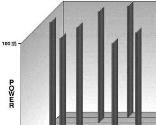
FHSS WLANs support 1 Mbps and 2 Mbps data rates. As the name implies, a FHSS device changes or “hops” frequencies with a predetermined hopping pattern and a set rate, as depicted in Figure 3-8. FHSS devices split the available spectrum into 79 nonoverlapping channels (for North America and most of Europe) across the 2.402 to 2.480 GHz frequency range. Each of the 79 channels is 1 MHz wide, so FHSS WLANs use a relatively fast 1 MHz symbol rate and hop among the 79 channels at a much slower rate.

Figure 3-8. Frequency Hopping Example

The hopping sequence must hop at a minimum rate of 2.5 times per second and must contain a minimum of six channels (6 MHz). To minimize the collisions between overlapping coverage areas, the possible hopping sequences can be broken down into three sets of length, 26 for use in North America and most of Europe. Tables 3-1 through 3-4 show the minimum overlap hopping patterns for different countries, including the U.S., Japan, Spain, and France.

In essence, the hopping patterns provide a slow path through the possible channels in such a way that each hop covers at least 6 MHz and, when considering a multicell deployment, minimizes the probability of a collision. The reduced set length for countries such as Japan, Spain, and France results from the smaller ISM band frequency allocation at 2.4 GHz.

FHSS PLCP

After the MAC layer passes a MAC frame, also known as a PLCP service data unit (PSDU) in FHSS WLANs, to the PLCP sublayer, the PLCP adds two fields to the beginning of the frame to form a PPDU frame. Figure 3-9 shows the FHSS PLCP frame format.

Figure 3-9. FHSS PPDU

The PLCP preamble consists of two subfields:

• The SYNC subfield is 80 bits long and is a string of alternating 0s and 1s, starting with 0. The receiving station uses the field to make an antenna-selection decision in diversity deployments, to correct any frequency offset, and to synchronize packet timing.

• The start of frame delimiter (SFD) subfield is 16 bits long and consists of a specific bit string (0000 1100 1011 1101, leftmost bit first) to provide frame timing to the receiving station.

The PLCP header consists of three subfields:

• The PSDU length word (PLW) is 12 bits long and specifies the size of the MAC frame (PSDU) in octets.

• The PLCP signaling field (PSF) is 4 bits long and indicates the data rate of the frame. Table 3-5 shows the decoding of the data rate.

• The header error control (HEC) is an International Telecommunications Union Telecommunication Standardization Sector (ITU-T) Cyclic Redundancy Check (CRC-16) value for the PLCP header field. The transmitter generates the checksum and then the receiver uses it to detect errors in the received PLW and PSF.

Table 3-5. PSF Decoding

b1	b2	b3	Data Rate
0	0	0	1.0 Mbps
0	0	1	1.5 Mbps
0	1	0	2.0 Mbps
0	1	1	2.5 Mbps
1	0	0	3.0 Mbps
1	0	1	3.5 Mbps
1	1	0	4.0 Mbps
1	1	1	4.5 Mbps

The PSDU is passed through a scrambler to whiten or randomize the input bit sequence, as described earlier in the section, “Physical Layer Building Blocks.” The resulting PSDU appears in Figure 3-10. Stuff symbols are also inserted between each 32-symbol block. These stuff symbols remove any bias in the data, more 1s than 0s or more 0s than 1s, which could have an undesirable effect upon later processing modules.

Figure 3-10. FHSS Scrambled PSDU

FHSS PMD-GFSK Modulation

The PLCP converts the frame into a binary bit stream and passes this bit stream to the PMD sublayer. The FHSS PMD sublayer modulates the data stream by using Gaussian frequency shift keying (GFSK).

To understand GFSK modulation, you must first grasp the basic concepts of Frequency Shift Keying (FSK). Unlike the QPSK modulation described earlier, FSK operates by representing each symbol with a different frequency. For example, if you want to convey the binary value 0, you transmit a sinusoid with a frequency of f₁; you transmit a frequency of f₂ for a binary value of 1. You agree upon the symbol period with your friend on the other side, and that would govern how long each sinusoid is transmitted. Often, rather than express the two frequencies in absolutes, you give them relative to the carrier frequency, f_c, specified in the hopping sequence. Figure 3-11 depicts a frequency domain of the frequencies with the magnitude given by the height of the vector, f₁ = f_c – f_d and f₂ = f_c + f_d.

Figure 3-11. FSK Frequency Domain Example

Some of the advantages of FSK are that you can fairly easily design a transmitter and receiver; in fact, FSK operates under the same principles as your FM radio receiver in your automobile. As you shall see in Chapter 8, FSK also greatly simplifies your radio-frequency design because it is a constant modulus signal, meaning that no information is carried by the amplitude of the signal, allowing you to transmit at a higher average power for a set peak power. However, FSK also has some significant disadvantages, not the least of which is that it is spectrally inefficient: It does not convey as much information per quantum of spectrum as other methods. In addition, the modulator is not a linear process, which means that it is difficult for you to correct the signal for channel impairments or to analytically determine the performance.

You can understand one of the great challenges for an FSK modulator by examining the transmission of a 0 followed by a 1. It requires the signal to instantaneously jump from a sinusoid of frequency f_c – f_d to a frequency of f_c + f_d, which introduces a discontinuous change in the transmitter output that creates significant amounts of out-of-band energy. Figure 3-12 shows an example of this challenge at baseband, meaning that the carrier component is removed.

Figure 3-12. FSK Frequency Transition

To combat this problem, you can filter the input to the frequency modulator to smooth the transition from f_c – f_d to f_c + f_d. For GFSK, you use a Gaussian filter, hence the name. f_d is referred to as the frequency deviation, and 802.11 specifies that it must be at least 110 kHz. For 2 Mbps operation, you use 4GFSK, which modulates two bits at a time using two deviation frequencies, as shown in Table 3-6, where f_d1 is roughly 3 times f_d2.

Table 3-6. 4 GFSK Symbol to Frequency Mapping

Symbol	Frequency
10	fc + fd2
11	fc + fd1
01	fc – fd1
00	fc – fd2

Although FHSS was fairly widely deployed in applications such as warehousing and manufacturing in the early days of WLAN, it does come with its own set of problems. The first and most basic is that it doesn't provide the kind of high data rates that are achievable in the wired LAN space and that the new WLAN standards offer. The second and slightly less obvious problem is that although up to 79 channels are available for use in the hopping sequence and each of the three standard hopping sets, as described in the beginning of this section, your signal will be hopping all over the ISM band, regardless of other energy and signals that might be in the band. As discussed in Chapter 8 and Chapter 9, “The Future of Wireless LANs,” no standardized method exists for you to eliminate those frequencies where there is known interference. If interference occurs in half of the band and you are operating at 1 Mbps, 50 percent of the time, you will be hopping to a channel that does not support communication because of the interference. So, your effective throughput will be 500 Kbps at most.

Even more interesting is that no mechanism exists to coordinate or synchronize the hopping sequences of adjacent access points. Their hopping sequences could overlap, causing more interference. If your bandwidth requirements are low and you do not need to scale to multiple access points, you can still deploy a limited network using FHSS.

DSSS is another physical layer for the 802.11 specifications. As defined in the 1997 802.11 standard, DSSS supports data rates of 1 and 2 Mbps. In 1999, the 802.11 Working Group ratified the 802.11b standard to support data rates of 5.5 and 11 Mbps. The 802.11b DSSS physical layer is compatible with existing 802.11 DSSS WLANs. The PLCP for 802.11b DSSS is the same as that for 802.11 DSSS, with the addition of an optional short preamble and short header.

DSSS WLANs use 22 MHz channels, which allows multiple WLANs to operate in the same coverage area. In North America and most of Europe, the use of 22 MHz channels allows for three nonoverlapping channels in 2.4 to 2.483 GHz range. Figure 3-13 shows these channels, which are discussed in more detail in Chapter 8.

Figure 3-13. DSSS Channelization

802.11 DSSS

Similar to the PLCP sublayer for FHSS, the PLCP for 802.11 DSSS adds two fields to the MAC frame to form the PPDU: the PLCP preamble and PLCP header. The frame format appears in Figure 3-14.

Figure 3-14. 802.11 DSSS PPDU

The PLCP preamble comprises two subfields:

• The SYNC subfield is 128 bits long and is a string of binary 1s. The function of the field is to provide synchronization for the receiving station.

• The SFD subfield is 16 bits long and consists of a specific bit string, 0xF3A0, to provide timing to the receiving station.

The PLCP header comprises four subfields:

• The Signal subfield is 8 bits long and specifies the modulation and data rate for the frame. Table 3-7 gives the mapping.

• The Service subfield is 8 bits long and is a reserved subfield, meaning that it was left undefined at the time the spec was written but also kept reserved so that future changes to the standard could use the subfield.

• The Length subfield is 16 bits long and contains the number of microseconds, ranging from 16 to 2¹⁶ – 1, that is required to transmit the MAC portion of the frame.

• The CRC subfield is 16 bits long and provides the resulting value of the same ITU-T CRC-16 used in FHSS as applied to the PLCP header subfields.

Table 3-7. Signal to Data Rate Mapping

Signal	Data Rate
0x0A	1 Mbps
0x14	2 Mbps

The PLCP converts the frame into a bit stream and passes the data to the PMD sublayer. The entire PPDU is passed through a scrambler to randomized the data.

The scrambled PLCP preamble is always transmitted at the 1 Mbps data rate, whereas the scrambled MPDU frame is transmitted at the data rate specified in the Signal subfield. The PMD sublayer modulates the whitened bit stream using one of the following modulation techniques:

• Differential binary phase shift keying (DBPSK) for 1 Mbps operation

• Differential quadrature phase shift keying (DQPSK) for 2 Mbps operation

The next section describes the DSSS PMD modulation process.

DSSS Basics

Spread-spectrum techniques take a modulation approach that uses a much higher than necessary spectrum bandwidth to communicate information at a much lower rate. Each bit is replaced or spread by a wideband spreading code. Much like coding, because the information is spread into many more information bits, it has the ability to operate in low signal-to-noise ratio (SNR) conditions, either because of interference or low transmitter power. With DSSS, the transmitted signal is directly multiplied by a spreading sequence, shared by the transmitter and receiver.

WLAN DSSS specifically encodes data by taking a 1 Mbps data stream from the data link layer and converting it to an 11 MHz chip stream. The spreading sequence (or chipping sequence or Barker sequence), which converts a data bit into chips, is an 11-bit value. In the case of 1 and 2 Mbps operation, one data bit is expanded to an 11-bit value. (A binary 1 expands to 1111111111 and 0 to 0000000000.) The expanded data bit is then exclusive ORed (XORed) with the spreading sequence, and the resulting chips are mapped to symbols and modulated. Figures 3-15 and 3-16 show this process.

Figure 3-15. Spreading a Data Bit with Value 1

Figure 3-16. Spreading a Data Bit with Value 0

You might wonder what good it does for WLANs to increase transmission overhead from 1 Mbps to 11 Mbps. The 11-chip sequence represents a single data bit. For example, suppose a chipped sequence is transmitted across the wireless medium. During the transmission, some interference occurs in a few of the channel's frequencies. Because the transmitter spreads the sequence across the 22-MHz–wide channel, only a few chips of the sequence should be impacted by the interference. The receiver is capable of rebuilding the original sequence by examining the received chips. Contrast this process to sending raw data bits, which incur data loss because of the interference and require subsequent retransmission. Direct sequencing can use the frequencies in a channel to increase throughput and reduce latency.

DBPSK Modulation

You might recall that we described QPSK symbol mapping or modulation onto the complex plane earlier in the section, “Physical Layer Building Blocks.” BPSK uses a similar technique, but each symbol has only an in-phase component because both constellation points reside on the I axis. Figure 3-17 shows the BPSK constellation.

Figure 3-17. BPSK Constellation

To ensure that the receiver does not need to remove the phase component of any frequency offset, the keying uses differential encoding, resulting in DBPSK. Differential encoding works as follows: Each chip maps into a single symbol. A 0 tells the symbol mapper to transmit the same symbol as in the previous symbol period, and a 1 tells the symbol mapper to rotate the phase by 180 degrees, or π in radians. BPSK also results in a constant modulus signal, thereby simplifying the radio design.

The PLCP sublayer for HR-DSSS has two PPDU frame types: long and short. The preamble and header in the 802.11b HR-DSSS long PLCP are always transmitted at 1 Mbps to maintain backward compatibility with DSSS. In fact, the HR-DSSS long PLCP is the same as the DSSS PLCP but with some extensions to support the higher data rates. These extensions are as follows:

The short PLCP PPDU provides a means to minimize overhead while still enabling transmitters and receivers to communicate appropriately. The 802.11b HR-DSSS short header, which is shown in Figure 3-18, still uses the same preamble, header, and PSDU format, but the PLCP header is transmitted at 2 Mbps, whereas the PSDU is transmitted at 2, 5.5, or 11 Mbps. In addition, the subfields are modified as follows:

Figure 3-18. HR-DSSS Short PPDU

Just like the 802.11 PHY, the PLCP converts the entire PPDU through the same scrambler used throughout 802.11 to the PMD. Within the PMD, the various subfields are transmitted at the appropriate data rate and modulation technique: CCK or PBCC.

Although the spreading mechanism to achieve 5.5 Mbps and 11 Mbps with CCK is related to the techniques you employ for 1 and 2 Mbps, it is still unique. In both cases, you employ a spreading technique, but for CCK, the spreading code is actually an 8 complex chip code, where a 1 and 2 Mbps operation uses an 11-bit code. The 8-chip code is determined by either four or eight bits, depending upon the data rate. The chip rate is 11 Mchips/second, so with 8 complex chips per symbol and 4 or 8 bits per symbol, you achieve the data rates 5.5 Mbps and 11 Mbps.

To transmit at 5.5 Mbps, you take the scrambled PSDU bit stream and group it into symbols of 4 bits each: (b0, b1, b2, and b3). You use the latter two bits (b2, b3) to determine an 8 complex chip sequence, as shown in Table 3-11, where {c1, c2, c3, c4, c5, c6, c7, c8} represent the chips in the sequence. In Table 3-11, j represents the imaginary number, sqrt(-1), and appears on the imaginary or quadrature axis in the complex plane.

Now with the chip sequence determined by (b2, b3), you use the first two bits (b0, b1) to determine a DQPSK phase rotation that is applied to the sequence. Table 3-12 shows this process. You must also number each 4-bit symbol of the PSDU, starting with 0, so that you can determine whether you are mapping an odd or an even symbol according to the table. You will also note that you use DQPSK, not QPSK, and as such, these represent phase changes relative to the previous symbol or, in the case of the first symbol of the PSDU, relative to the last symbol of the preceding 2 Mbps DQPSK symbol.

Apply this phase rotation to the 8 complex chip symbol and then modulate that to the appropriate carrier frequency.

To transmit at an 11 Mbps data rate, you group the scrambled PSDU bit sequence into 8 bit symbols. The latter 6 bits select one 8 complex chip sequence, out of 64 possible sequences, much the same way that bits (b2, b3) were used to select one sequence from four possible. You use bits (b0, b1) in the same manner as 5.5 Mbps CCK to rotate the sequence and then modulate it to the appropriate carrier frequency.

As already indicated, the HR-DSSS standard also defines an optional PBCC modulation mechanism for generating 5.5 Mbps and 11 Mbps data rates. This scheme is a bit different from both CCK and 802.11 DSSS. You first pass the scrambled PSDU bits through a half-rate binary convolution encoder, which was first introduced in the section, “Physical Layer Building Blocks.” The particular half-rate encoder has six delay, or memory elements, and outputs 2 bits for every 1 input bit. Because 802.11 works under a frame structure and convolutional encoders have memory, you must zero all the delay elements at the beginning of a frame and append one octet of zeros at the end of the frame to ensure all bits are equally protected. This final octet explains why the length calculation, discussed in the section, “802.11b HR-DSSS PLCP,” is slightly different for CCK and PLCC. You then pass the encoded bit stream through a BPSK symbol mapper to achieve the 5.5 Mbps data rate or through a QPSK symbol mapper to achieve the 11 Mbps data rate. (You do not employ differential encoding here.) The particular symbol mapping you use depends upon the binary value, s, coming out of a 256-bit pseudo-random cover sequence. The two QPSK symbol mappings appear in Figure 3-19, and the two BPSK symbol mappings appear in Figure 3-20. For PSDUs longer than 256 bits, the pseudo-random sequence is merely repeated.

Figure 3-19. PBCC QPSK Symbol Mapping

Figure 3-20. PBCC BPSK Symbol Mapping

The IEEE 802.11j draft amendment for LAN/metropolitan-area networks (MAN) requirements provides for 802.11a type operation in the 4.9 GHz band allocated in Japan and in the U.S. for public safety applications as well as in the 5.03 to 5.091 GHz Japanese allocation. A channel numbering scheme uses channels 240 to 255 to cover these frequencies in 5 MHz channel increments.

The PLCP sublayer for the 802.11a PHY has its own unique PPDU frame format, which is shown in Figure 3-21.

Figure 3-21. 802.11a PPDU Frame Format

Three basic pieces make up the PPDU: OFDM preamble, Signal, and Data. The OFDM preamble consists of short SYNC training sequences and a long sync training symbol. The receiver uses the former for automatic gain control (AGC), timing, and initial frequency offset estimation, whereas it uses the latter for channel, timing, and fine frequency offset estimation. The mechanism for constructing this is discussed later in this section.

You compose the Signal field with five subfields:

The Data field contains four subfields:

To understand the “how” and “why” of the 802.11a OFDM PMD, you first need to understand the basics of OFDM, which is unlike any modulation technique discussed so far. OFDM is part of a family of multichannel modulation schemes that were invented to transmit data under severe intersymbol interference (ISI). Consider the simple QPSK symbol first introduced in the section, “Physical Layer Building Blocks,” and then consider the transmission of two consecutive symbols. As these symbols travel through the transmission medium from the transmitter to the receiver, they experience distortions, and various parts of the signal can be delayed. If these delays are long enough, the first symbol might overlap in time with the second symbol. This overlapping is ISI. The time delay from the reception of the first instance of the signal until the last instance is referred to as the delay spread of the channel. You can also think of it as the amount of time that the first symbol spreads into the second. Traditionally, designers address ISI in one of two ways: employing symbols that are long enough to be decoded correctly in the presence of ISI or by equalizing to remove the distortion caused by the ISI. The former method limits the symbol rate to something less than the bandwidth of the channel, which is inversely proportional to the delay spread. As the bandwidth of the channel increases, you can increase the symbol rate, thereby achieving a higher end data rate. The latter method, often used in conjunction with the former, requires the use of ever more complicated and expensive methods to implement channel-equalization schemes to maximize the usable bandwidth of the channel.

Multichannel modulation schemes take a completely different approach. As a multichannel modulation designer, you break up the channel into small, independent, parallel or orthogonal transmission channels upon which narrowband signals, with a low symbol rate, are modulated, usually in the frequency domain, onto individual subcarriers. Similar to how you can modulate FHSS signal onto the appropriate carrier, you break the channel into N independent channels. For a given channel bandwidth, the larger the N that you choose, the longer the symbol period and the narrower the subchannel, so you can see that as the number of subchannels goes to infinity, the ISI goes to zero.

To build these independent symbols, a useful tool is the Fast Fourier Transform (FFT), which is an efficient implementation of a Discrete Fourier transform (DFT) and can convert a time domain signal to the frequency domain and vice versa. In the frequency domain, you generate N 4-QAM (Quadrature Amplitude Modulation) symbols, which are then converted to the time domain using an inverse FFT (IFFT). You should also know that making the size of the FFT a power of two allows for simple and efficient implementations. For that reason, OFDM systems usually pick N such that it is a power of two.

Without going into the intricacies of mathematics that are beyond the scope of this book, it simplifies the processing greatly if everything is done in the frequency domain using FFTs. To enable this processing at the receiver, however, the received signal must be a circular convolution of the input with the channel, as opposed to just a convolution. Convolution is a mathematical mechanism for passing a signal through a channel and determining the output. To ensure this property, you must take the time domain representation of an OFTM symbol and create a cyclic prefix by repeating the final ν samples at the beginning. Figure 3-22 shows this process, where ν is the length of the cyclic prefix and N is the size of the FFT in use.

Figure 3-22. OFDM Cyclic Prefix Formation

The length of the cyclic prefix must be longer than the delay spread of the channel to ensure that each OFDM symbol received is a circular convolution of the channel with the transmitted symbol. Another way to think about it is that you want a guard time between symbols, which ensures that any residual signal from the previous OFDM symbol has died off before you perform your processing on the current symbol. This time allows for symbol-by-symbol processing, and when it happens in the frequency domain, it allows for subchannel-by-subchannel processing.

To allow the receiver to estimate the channel, you often either intersperse known training symbols on some of the N subcarriers or transmit a separate known OFDM symbol that the receiver can use to estimate the channel. You also often fill the subchannels at the band edges with 0s to aid the transmitter because the filters in the transmitter and receiver will most likely attenuate them to the point where no information could be carrier over them anyway.

Unlike some other multichannel modulation techniques, OFDM places an equal number of bits in all subchannels. In nonwireless applications such as asynchronous digital subscriber line (ADSL), where the channel is not as time varying, the transmitter uses knowledge of the channel and transmits more bits, or information, on those subcarriers that are less distorted or attenuated.

As previously mentioned, the SYNC consists of long and short symbols, as depicted in Figure 3-23. Ten short training symbols exist, each of which is a short OFDM symbol that fills 12 of the 52 usable subchannels with a specified QPSK symbol in multiples of 4. It results in a periodic time domain sequence that you can use for detecting the start of the frame, performing automatic gain control, selecting the appropriate antenna if selection diversity is in use, estimating coarse frequency offset, and synchronizing the timing.

Figure 3-23. SYNC Field

The two long training symbols are identical and modulate the subcarriers by a specific sequence. The long training sequences allow you to perform channel estimation and fine frequency offset estimation. Because they are designed to be processed together, they require only a single guard interval, indicated by G in Figure 3-23.

Figure 3-24 depicts the generalized OFDM transmitter used by the 802.11a OFDM PMD. As in other PHY schemes, you pass the data bits through the scrambler and then through a convolution encoder to create coded bits. The rate is determined by the data rate in use. Next, you interleave the coded bits in groups that are equal in size to the number of coded bits per OFDM symbol. The interleaved coded bits are then mapped into 48 symbols with the number of bits per symbol determined by the data rate. These are placed into 48 of the subcarriers of the OFDM symbol, and pilot tones are placed into 4 of the subcarriers. An IFFT is performed and is followed by the formation of the cyclic prefix. The resulting sequence is modulated to the appropriate carrier.

Figure 3-24. 802.11a Generalized OFDM Transmitter

Table 3-14 shows how the data rate is mapped to the appropriate parameters for the components of the OFDM transmitter.

The Signal field described earlier is transmitted in a single OFDM symbol at the 6 Mbps data rate, which allows the transmission of 24 data bits. This explains why there are 6 Tail bits at the end of the field. The Data field is transmitted as a number of sequential OFDM symbols, at the data rate specified in the Rate subfield of the Signal field. You can determine the number of pad bits required to make the length of the Data field a multiple of the number of coded bits per OFDM symbol once you know the length of the PSDU.

Examining the details of the 802.11a transmitter, the scrambler uses the same generator polynomial that is used in all the other 802.11 modulation schemes. The convolutional encoder uses a slightly different base rate 1/2 encoder than you would use for the optional 802.11b PBCC. The rate 2/3 and 3/4 encoders are formed by puncturing or omitting some of the encoded bits at the transmitter and then replacing them with 0 bits at the receiver. This replacement has the end effect of increasing the coding rate because there are fewer coded bits transmitted per input bits. The puncturing is performed in a known and systematic manner.

The interleaver is a block interleaver with the block size given by the number of coded bits per OFDM symbol. The interleaving actually occurs in two steps.

The first step ensures that adjacent coded bits are mapped into nonadjacent subcarriers, whereas the second step ensures the adjacent coded bits are mapped in an alternating pattern into less and more significant bits of the constellation symbol mapping. This process is important because in higher order constellations, the least significant bits (LSBs) are often less reliable. The issues is more evident when you examine the constellations, where constellation points that are close together and more easily confused or mistaken tend to only differ in their LSBs.

The mappings of groups of bits into symbols in the complex plane appear in Figures 3-25, 3-26, 3-27, and 3-28 for BPSK, QPSK, 16-QAM, and 64-QAM, respectively.

Figure 3-25. 802.11a BPSK Constellation

Figure 3-26. 802.11a QPSK Constellation

Figure 3-27. 802.11a 16-QAM Constellation

Figure 3-28. 802.11a 64-QAM Constellation

To make sure that all data rates statistically have the same average power, each symbol is multiplied by a scaling factor that is a function of the modulation type. Table 3-15 gives the scale factor.

Within each OFDM symbol, four pilot signals are also added at regular intervals in the IFFT for use by the receiver. These pilot subcarriers are BPSK encoded and modulated by a pseudo binary sequence.

The 802.11g standard defines five PPDU formats: long preamble, short preamble, ERP-OFDM preamble, a long DSSS-OFDM preamble, and a short DSSS-OFDM preamble. Support for the first three is mandatory, but support for the latter two is optional. Table 3-16 summarizes the different preambles and the modulation schemes and data rates they support or are interoperable with.

The long preamble uses the same long preamble defined in the HR-DSSS but with the Service field modified as shown in Table 3-17.

The length extension bits determine the number of octets, when the 11 Mbps PBCC and 22 and 33 Mbps ERP-PBCC modes are in use.

The short preamble makes the same modifications to the HR-DSSS short preamble that are summarized in Table 3-16.

The ERP-OFDM preamble takes the 802.11a preamble and adds an extra 6 microsecond signal extension, during which no transmission occurs, to make the packet longer to align it with the longer 16 microsecond SIFS timing of 802.11a versus the 10 microsecond SIFS timing of 802.11b.

The CCK-OFDM Long Preamble PPDU format appears in Figure 3-29. You set the rate subfield in the Signal to 3 Mbps. This setting ensures compatibility with non-ERP stations because they still read the length field and defer, despite not being able to demodulate the payload. The PLCP header matches that of the previously defined long preamble, but the preamble is the same as for the HR-DSSS. Both the preamble and the header are transmitted at 1 Mbps using DBPSK, and the PSDU is transmitted using the appropriate OFDM data rate. The header is scrambled using the HR-DSSS scrambler, and the data symbols are scrambled utilizing the 802.11a scrambler.

Figure 3-29. CCK-OFDM Long and Short Preamble PPDU Format

Much like the DSSS-OFDM long preamble, the short preamble DSSS-OFDM PPDU format uses the HR-DSSS short preamble and header at a 2 Mbps data rate. With the HR-DSSS scrambler and the data symbols, the short preamble and header are transmitted with OFDM and use the 802.11a scrambler.

As previously stated, the ERP-OFDM provides a mechanism to use the 802.11a data rates in the ISM band in a manner that is backward compatible with DSSS and HR-DSSS. In addition to utilizing the 802.11a OFDM modulation under the 2.4 GHz frequency plan, ERP-OFDM also mandates that the transmit center frequency and symbol clock frequency are locked to the same oscillator, which was an option for DSSS. It utilizes a 20 microsecond slot time, but this time can be dropped to 9 microseconds if only ERP devices are found in the BSS.

The higher data 22 and 33 Mbps PBCC data rates use the same mechanism as the lower rate 5.5 and 11 Mbps PBCC, but with 8-PSK instead of QPSK and BPSK to get 22 Mbps. 33 Mbps is achieved by using a 16.5 MHz clock instead of 11 MHz. The symbol mapping, as governed by the cover sequence, appears in Figure 3-30.

Figure 3-30. 802.11g ERP-PBCC Constellation

The key item to remember about 802.11g: It extends the data rates supported at 2.4 GHz up to 54 Mbps in a manner that ensures backward compatibility with older 802.11b devices. In an environment with only 802.11g devices operating, all transmissions take place at the highest data rates available. However, as soon as an 802.11b device is introduced, the header information needs to back down to the 802.11b rates that this older device can understand. This backing down occurs on all transmissions regardless of whether they are between 802.11g or 802.11b devices. The end effect is an overall increase in overhead, so a small price is paid for the backward compatibility that 802.11g affords.