
Although it is one thing to understand the basic components of the 802.11 physical layers (PHYs), it is an entirely different task to understand when and where you can deploy wireless LANs (WLANs) and what limitations and regulations govern their deployment. As mentioned in Chapter 3, “802.11 Physical Layer Technologies,” the use of unlicensed frequencies is one of the major enabling factors that has allowed WLANs in nearly every business segment. This chapter examines the rules that you need to know when planning your wireless deployment. It is also important to know the challenges that the radio designer faces, and although this chapter will not help you design an 802.11 radio, it will help you understand and evaluate the physical layer data that is presented by most equipment vendors. Every radio has a transmitter and a receiver; this chapter explains the basic performance parameters of these components. Armed with this knowledge, you can make intelligent and measured evaluations of the radios and antennas on the market.
The term radio refers to electromagnetic transmission through free space at millimeter wave frequencies and below. It encompasses a wide range of applications, from AM and FM car radios to cellular phone radios and terrestrial digital microwave radios. Some, like AM and FM radios, are one-way or broadcast radios. The electromagnetic transmission occurs in only one direction, and it is often in a one-to-many type configuration. Alternatively, two-way radios allow transmission and reception by all parties; they can either be a point-to-point configuration, which is common in telecommunications backhaul applications, or a point-to-multipoint configuration, such as WLAN and cellular networks.
An important architectural distinction with two-way radio communication is the difference between frequency division duplex (FDD) and time division duplex (TDD). In FDD, you use a different frequency to carry information in each direction, and the two frequencies are separated enough in frequency that they don't interfere. Provided adequate separation is maintained, FDD can significantly simplify the radio and system designer's task, and it allows full-duplex type operation where simultaneous transmission and reception can occur. However, it also suffers the problem that you must allocate spectrum in two bands, and it can be spectrally inefficient because it locks up bandwidth in each direction. The alternative, TDD, does all radio communication on the same channel but with alternating periods of transmitting and listening. Although TDD does create a half-duplex situation at the physical layer and does require the radio to be able to very quickly switch from transmitting to receiving, it can be more spectrally efficient. It allows for easier channelization, and it can provide for time-varying allocation of bandwidth in each direction.
One of the most important characteristics of a radio is power. Specifically, the output power of the radio is presented to the transmission line, cable, or antenna and is usually measured in watts or milliwatts (mW). Comparisons of power values use a logarithmic scale to express the ratio in decibels (dB). The radio manufacturer provides the output power in dBm, which is decibels per 1 mW, or in dBW, which is decibels per 1 W. Table 7-1 provides some sample conversions between powers in watts and decibels.
What is an antenna? The IEEE defines an antenna as “that part of a transmitting or receiving system that is designed to radiate or receive electromagnetic waves” (IEEE Standard 145-1993). In other words, it is the antenna that takes the radio frequency (RF) signal that the radio generates and radiates it into the air or that receives or captures electromagnetic waves for the radio. Usually, the transmit and receive properties are reciprocal, meaning that the parameters such as gain or radiation pattern or frequency are the same.
The next question you might ask is, “How does an antenna work?” According to the textbook that most antenna designers learned with—Stutzman and Thiele's Antenna Theory and Design—the key is radiation, a “disturbance in the electromagnetic field that propagates away from the source of the disturbance…disturbance is created by a time-varying current source.” So the radio creates a time-varying voltage source at a particular frequency, which induces a time-varying current on the antenna that creates the aforementioned electromagnetic field.
Considerations of antenna performance make a distinction between the near field, close to the antenna, and the far field. In the far field, the distance from the antenna is much larger than the wavelength at which you are operating or much larger than the dimension of the antenna, in contrast to the near field. It is under far-field assumptions that antenna vendors specify the characteristics of the antenna. Keep this point in mind if you ever find yourself operating in the near field of antennas because the characteristics are different.
An important concept to understand is that of an isotropic radiator or antenna. It is a mathematical construct for an idealized lossless antenna that radiates equally in all directions. If you define a sphere with an isotropic radiator in its center, the electromagnetic field will be equal at all points on the surface of the sphere. The isotropic antenna is a useful reference point when we consider different antennas.
For you to make a judicious antenna decision, it is important to understand some of the properties that describe an antenna. They include, but are not limited to, an antenna's radiation pattern, directivity, gain, input impedance, polarization, and bandwidth.
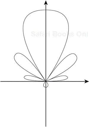
The radiation pattern of an antenna describes the “angular variation of radiation at a fixed distance from an antenna.” It is often expressed in terms of directivity or gain. The directivity of an antenna describes the intensity of the radiation in a given direction, relative to the average radiation intensity, or put another way, it indicates the radiated power density relative to a uniformly distributed radiated power. Gain expresses the same concepts as directivity, but it also includes losses on the antenna itself. You can define radiation efficiency that is used to scale the directivity to determine the gain; a perfect radiator has a radiation efficiency of 1. As all real antennas have losses, gain is the more frequently quoted parameter for an antenna. The units used to describe the gain are either dBi, gain in dB relative to an isotropic antenna, or dBd, gain in dB relative to a half-wave dipole antenna. To convert between dBd and dBi, merely add 2.2 to the gain expressed in dBd to get the gain in dBi. This conversion is important for you to remember because although most vendors express gain in dBi, some express it in dBd. Figure 7-1 shows a sample radiation pattern for a directional antenna.
NOTE
You can construct a dipole antenna by taking a transmission line and bending the ends outward to create oppositely charged poles that induce a time-varying current between them.
Remembering that this radiation exists in three-dimensional space, you often find that an antenna has a main lobe or beam, which is the direction of maximum gain, and that it is also characterized by minor lobes, often referred to as side and backlobes, depending upon the direction of the minor lobe relative to the main lobe. Vendors often describe antennas by the gain of the main lobe. When doing so, they also specify the beamwidth of the antenna. It is usually the principle half-power beamwidth, which is defined by the IEEE as follows: “In a radiation pattern cut containing the direction of the maximum of a lobe, the angle between the two directions in which the radiation intensity is one-half the maximum value.” Take the previous antenna pattern and go to the points on either side of the main lobe where the gain is 3 dB lower than the maximum point of the lobe; this point is the half-power point, and it is where the angle between them gives the half-power beamwidth. Figure 7-2 illustrates this description.
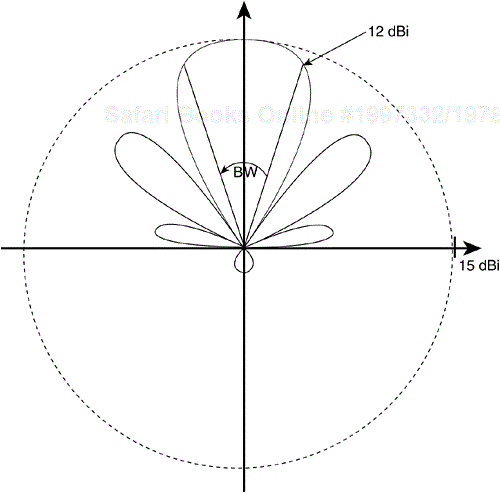
Related to an antenna's radiation pattern, the front-to-back ratio of an antenna compares the maximum gain of an antenna on its main lobe to the gain on a rearward facing lobe. In the sample radiation pattern, the front-to-back ratio is 20 dB, as shown in Figure 7-3. The main lobe gain is 15 dBi, and the back lobe is -5 dBi. The difference, 15 dBi…(-5 dBi) = 20 dB, is the front-to-back ratio.

Now that you understand the gain of an antenna, it is time to examine the actual power that is transmitted by a radio connected to an antenna. The effective radiated power (ERP) takes the gain of an antenna in units of dBd, relative to a half-wave dipole, and multiplies it by the net power offered by the transmitter to the antenna. However, you most often perform this operation in the log, or dB, domain, which means you add the gain of the antenna to the transmitter power. Because it is more common to express the gain of an antenna in dBi units, the more commonly used term for radiated power is effective isotropic radiated power (EIRP), which is the same as ERP but with the antenna gain expressed relative to an isotropic radiator.
The electromagnetic waves emitted by an antenna can trace different patterns that affect propagation. The pattern depends upon the polarization of the antenna, which could be linearly or circularly polarized.
Most antennas that you find for WLANs are linearly polarized, either horizontal or vertical. In the former case, the electric field vector lives in the vertical plane, and in the latter the plane is horizontal. Vertical polarization is more common, although you might find scenarios where horizontal polarization works better. Although it isn't likely that you will use circularly polarized antennas indoors, using wireless bridging technology you might find applications for them. As with linearly polarized antennas, there are two cases: left-hand polarized and right-hand polarized. If the vector rotates clockwise as the wave is traveling toward you, then it is left-hand polarized.
Similarly, if it rotates counter-clockwise, it is right-hand polarized. Shooting a link over a body of water, where the polarization can rotate with each reflection, is an example of where circular polarization would be useful because it is invariant with respect to rotation. A linearly polarized antenna could switch from vertical to horizontal as it rotates.
In general, for a line-of-sight link, you should use the same polarization on both sides. A 21 dBi vertically polarized antenna might have only 1 to -4 dBi of gain in the horizontal plane; that is, the cross-polarization discrimination is typically 20 to 25 dB.
The radiation efficiency of an antenna is “the ratio of the total power radiated by an antenna to the net power accepted by the antenna from the connected transmitter.” The antenna radiates some power as electromagnetic energy. All RF devices—radios, transmission lines, or antennas—have a characteristic impedance, which is the ratio of the voltage to the current at their terminal. With an antenna connected to a cable, if the antenna input impedance matches the radio and transmission-line impedance, then the maximum amount of power is transferred from the radio to the antenna. However, if there is an impedance mismatch, some of the energy is reflected back in the direction of the source, and the remainder is transferred to the antenna. The voltage standing wave ratio (VSWR) characterizes these reflections. If no reflections exist, the VSWR equals 1. As the VSWR increases, there are more reflections of greater magnitude. A VSWR of 2 means that 11 percent of the power is reflected.
A high VSWR and a lossy transmission line loses or wastes significant energy. Even more unsettling: With a high VSWR and high powers, a dangerous situation can develop as high voltages build up on the transmission line and, in extreme cases, cause arcing. However, this situation should never be an issue for you at the low power levels of your WLAN deployments.
The bandwidth of an antenna defines the range of frequencies over which the antenna provides acceptable performance, usually defined by the upper or maximum frequency and the lower or minimum frequency. Acceptable performance in this case means that characteristics of the antenna, such as the antenna pattern and the input impedance, do not change over the operating range of frequencies. Some antennas are considered broadband, which is loosely defined as those antennas for which the ratio of the maximum frequency to the minimum frequency is greater than 2. However, because broadband antennas often have poor gain performance and because the currently allocated 802.11 WLAN frequencies do not require a broadband antenna, the only instance in which you might be offered a broadband antenna is if you want to cover the entire 2.4 GHz Industrial, Scientific, and Medical (ISM) band along with the 5 GHz Unlicensed National Information Infrastructure (U-NII) band with a single antenna.
Remember when you make your antenna choices that many of the antenna properties are interrelated, so that although it might seem optimal to maximize or minimize all the antenna's characteristics, this task is often not possible. For example, if you select a very wide beamwidth, you sacrifice gain; if you select a broadband antenna, you might find that the antenna pattern is not uniform. So it is important to determine what characteristics are important for your particular deployment and optimize your choice accordingly.
You will come across many types of antennas in your lifetime. Rather than list all of them, this section describes the types of antennas that you are most likely to find in WLAN applications. Figure 7-4 shows several different types of antennas. As previously mentioned, an isotropic radiator is an idealized nonrealizeable antenna that has a uniform radiation pattern in all directions.
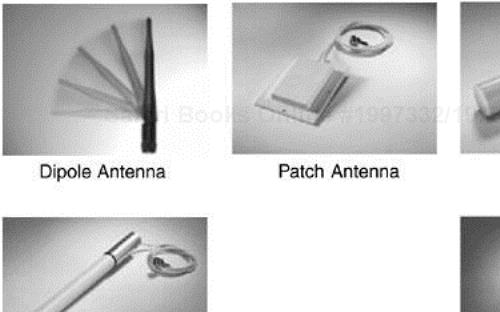
With a half-wave dipole, the length from end to end is equal to half the wavelength at that frequency. An omnidirectional antenna provides uniform gain in all directions on a plane, often the horizontal plane. Dipole antennas are usually omnidirectional. Omnidirectional antennas are typically used in general WLAN deployments because they provide coverage in all directions. A Yagi-Uda antenna is constructed by forming an linear array of parallel dipoles.
Yagi antennas are some of the more common directional antennas because they are so easy to build. Directional antennas, such as Yagis, typically provide coverage in hard-to-reach areas or where more range is needed than an omnidirectional antenna can provide.
Patch antennas, another type of directional antenna, are formed by placing two parallel conductors with a substrate between them. The upper conductor is a patch that can be simply printed on a circuit board. It is relatively simple to form an array of patches, the antenna patterns of which combine to form various directed beam shapes. Patch antennas are often useful because of their rather slim profile, in contrast to that of a Yagi antenna. In the broad category of directional antennas are broadside antennas, in which the main beam is perpendicular to the plane of the antennas; end fire antennas, in which the main beam is in the plane of the antenna; and pencil beams, which provide a single, very narrow and often high-gain lobe to the antenna.
Chapter 10, “WLAN Design Considerations,” discusses the circumstances under which you might use each type of antenna.
Radio receivers are characterized by their receiver sensitivity, which is the minimum signal level for the receiver to be able to acceptably decode the information. The acceptability threshold is governed by a particular bit error rate (BER), packet error rate (PER), or frame error ratio (FER). For example, the 802.11a standard specifies that the minimum compliant receiver performance at a 54 Mbps data rate is –65 dBm at a 10 percent PER. Note that the receiver sensitivity is also at a specific data rate because each modulation scheme has its own signal-to-noise ratio (SNR) requirement. In general, the higher the data rate, the higher the SNR required and hence the higher the receiver sensitivity level. The receiver sensitivity of the radio is also governed by the receiver noise figure. All receivers have some base underlying noise level, either from the precision of the digital processing or from the performance of the analog components. This noise level is the noise floor. As the noise floor rises, so too does the receiver sensitivity because the minimum signal level over the noise, SNR, is fixed for the modulation scheme. This concept is depicted in Figure 7-5. To evaluate the performance of a radio, receiver sensitivity is one of the important inputs to your link-budget calculation that ultimately determines the achievable data rates and ranges. In general, you want the lowest receiver sensitivity that is economically feasible.
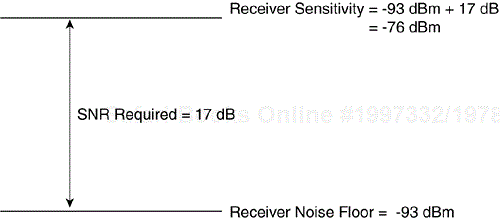
To ensure satisfactory system performance between equipment manufactured by different vendors, the 802.11b PHY standard defines minimum radio performance levels that all equipment must satisfy for compliance. At an FER less than .08 with a Physical Layer Convergence Procedure service data unit (PSDU) length of 1024 octets at an 11 Mbps data rate, the minimum receiver sensitivity is –76 dBm at the antenna connector. Under the same conditions, the receiver maximum input level is –10 dBm at the antenna connector, and the adjacent channel rejection of another compliant 802.11b transmitter is 35 dB at the antenna connector. For adjacent channel rejection, the receiver must be able to adequately filter or operate in the presence of an adjacent signal to maintain the 0.08 FER. To test adjacent channel rejection, the desired signal is placed 6 dB over the minimum receiver sensitivity level, and the adjacent channel signal is placed 41 dB over that same level. In the discussion of the 802.11b spectral mask, you will see what the likely resultant channel signal contribution is from the interferer.
Similar to 802.11b, 802.11a also defines minimum radio performance parameters. Table 7-2 provides the minimum receiver sensitivity, adjacent channel rejection, and alternate adjacent channel rejection at the antenna connector for the 802.11a data rates at a PER less than 10 percent with a 1000-byte PSDU length. In the rejection performance, the desired signal is placed 3 dB over the minimum sensitivity level and the interferer at the level given by the ratio indicated.
Table 7-2. Minimum 802.11a Minimum Radio Performance
Data Rate (Mbps) | Minimum Sensitivity (dBm) | Adjacent Channel Rejection (dB) | Alternate Adjacent Channel Rejection (dB) |
|---|---|---|---|
6 | -82 | 16 | 32 |
9 | -81 | 15 | 31 |
12 | -79 | 13 | 29 |
18 | -77 | 11 | 27 |
24 | -74 | 8 | 24 |
36 | -70 | 4 | 20 |
48 | -66 | 0 | 16 |
54 | -65 | -1 | 15 |
The receiver maximum input level under the same conditions is –30 dBm. 802.11a also specifies the clear channel assessment (CCA) sensitivity, which states that a compliant radio must indicate busy with 90 percent probability within 4 microseconds if the received level is greater than or equal to –82 dBm during the preamble. If the preamble is missed, then the level is –62 dBm.
Ultimately, what concerns you and the users of your WLAN network from a radio performance perspective is coverage and throughput. They are directly related to the range at each data rate. To determine the range, you must know how to translate from the system gain that you can provide to the corresponding range in your environment. Under free space, line-of-sight conditions, this process is relatively straightforward because the path loss is proportional to the square of the distance or range. The range is that distance at which the path loss equals the system gain. In other words, you require 6 more dB each time you double your distance. However, the typical indoor WLAN environment is cluttered with walls, desks, people, and other objects, all of which degrade the signal and increase the loss. As Chapter 8, “Deploying Wireless LANs,” discusses, the only way to get an accurate understanding of the path loss in your environment is to conduct a site survey. However, it is still useful to understand the mechanisms that affect system performance and how to determine your system gain for comparison with other systems.
A link budget is the tool that you can use to determine the overall system gain. You need to know the following pieces of information for you system:
Radio transmit power
Transmit cable loss, if any
Transmit antenna gain
Receiver antenna gain
Receiver cable loss, if any
Receiver sensitivity at the desired data rate
The cable loss is a function of the frequency and should be provided in the cable specification by the vendor. In general, as frequencies increase, so too does cable loss, so you want to be more careful with remote antennas and long RF cable runs in the U-NII bands than in the 2.4 GHz ISM band. For example, a 100-foot cable run of LMR-400, a fairly common low-loss RF cable, has a cable loss of 10.5 dB at 5.3 GHz but only 6.5 dB at 2.4 GHz.
If you multiply the transmit power and the antenna gains and then divide by the cable losses and receiver sensitivity, you get the overall system gain:
Alternatively, if you perform the operations in the log or dB domain, it is merely a matter of addition and subtraction:
System GaindB = PTx + GTx + GRx – (LTx + LRx + SRx)
Table 7-3 provides two sample link budgets using hypothetical radios at 2.4 GHz with a 50-foot cable run at the access point (AP) in both cases. The table provides both the down-stream, AP to client, and upstream, client to AP, link budgets for both systems. System B uses a lower-performing AP with lower transmit power and higher receive sensitivity. You can see that in the downstream, system B is 3 dB worse than system A, but in the upstream, it is 11 dB worse. For system A, the downstream limits the overall range and data rate, but for system B is limited by the upstream. In a free-space environment, system A would have a 5 dB link-budget advantage, resulting in nearly twice the range at the same data rate. Each 6 dB increase in link budget doubles the range in free space. In this way, you can see that you must consider the overall system gain when evaluating the coverage and throughput that two wireless systems can provide.
Table 7-3. Sample Link Budget
System A Downstream | System A Upstream | System B Downstream | System B Upstream | |
|---|---|---|---|---|
Transmit Power (dBm) | 20 | 15 | 17 | 15 |
Transmit Cable Loss (dB) | 3.3 | 0 | 3.3 | 0 |
Transmit Antenna Gain (dB) | 6 | 2 | 6 | 2 |
EIRP (dBm) | 22.7 | 17 | 19.7 | 17 |
Receiver Antenna Gain (dB) | 2 | 6 | 2 | 6 |
Receiver Cable Loss (dB) | 0 | 3.3 | 0 | 3.3 |
Receiver Sensitivity (dBm) | -76 | -87 | -76 | -76 |
System Gain (dB) | 100.7 | 106.7 | 97.7 | 95.7 |
As previously mentioned, other mechanisms also influence the performance of your system. They include, but are not limited to, the following:
Interference
Multipath
Fading
Interference occurs when some other signal source is producing energy on the channel in which you are trying to operate. It could be another WLAN radio operating on the same channel or some other device that produces energy in the same band. The stronger this source of interference, the stronger your receive signal level must be to decode the desired signal. You can think of it as raising the receiver sensitivity much the same way that raising the noise floor does, and if the undesired signal is too strong, you might not be able to operate at all. This effect is shown in Figure 7-6.

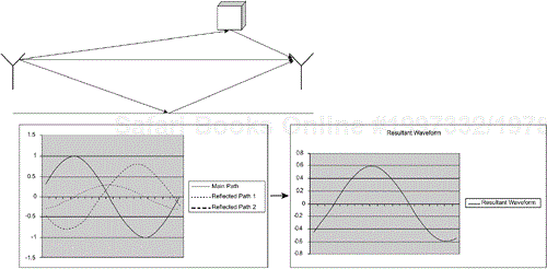
Multipath occurs when the desired signal reaches the receiving antenna via multiple paths, each of which has a different propagation delay and path loss. These different paths are usually caused by reflections off objects in the environment or off inhomogeneous atmospheric conditions. Each of these received paths are summed at the antenna, and depending upon the delays and the attenuation of each path, multipath fading can occur. Figure 7-7 shows an example of summing the different multipath rays.
Fading is a time-varying change in the path loss of a link with the time variance governed by the movement of objects in the environment, including the transmitter and receiver themselves. For example, you might be sitting in a conference room with a wireless laptop and be connected to an AP in the hallway. If someone closes the door to the conference room, the path loss drops, resulting in a lower received signal level. This scenario is a fade.
Flat fading occurs when the entire signal across the whole channel fades. With broadband signals like 802.11, frequency-selective fading can also occur. The signal might be significantly attenuated at certain frequencies but not at others. If you think back to orthogonal frequency-division multiplexing (OFDM), you will recall that it independently energizes individual frequencies and then codes and interleaves across them. This process provides OFDM with a distinctive advantage over other modulation schemes like Complementary Code Keying (CCK) in that if a frequency selective fade occurs, it might only attenuate a few tones of an OFDM signal, thereby allowing the coding and interleaving to restore the original bit stream. With CCK, the entire bit stream might be lost.
Depending upon the multipath characteristics, it can change the path-loss model from that of free space, which is proportional to the square of the distance, to a path loss that is proportional to the fourth power of the distance. Under these circumstances, the path loss would increase by 12 dB (10*log(244)=12) instead of 6 dB (10*log(222)=6) every time the distance is doubled. In other words, if you are communicating in an environment with full line of sight between the transmitter and receiver and no clutter to reflect or absorb energy, you need to add 6 dB to your link budget to double the range. However, for a large number of multipath reflectors, you might need to add 12 dB to your link budget to double the range.
The multipath profile is not only time varying, but it is also a function of location. Points in space that are very close to each other can experience very different fades (i.e., multipath spatial variation). You have experience with this phenomenon in your everyday life when sitting at a traffic light listening to your car radio, you roll forward or backward a few inches only to discover drastically different reception. This spatial variation in multipath is one of the main reason why WLANs employ multiple or diversity receive and transmit antennas. If these antennas are separated by at least a wavelength, then the signals they receive become uncorrelated, so when one is experiencing a fade, the other might not. Most WLAN devices use selection diversity in which the radio determines which antenna is receiving the better signal, and then uses that signal.
The Federal Communications Commission (FCC) has regulatory control over the wireless spectrum in the United States. Although many countries have similar spectrum regulations, unlicensed wireless can vary by country and continent. This section highlights the major spectrum regulations.
In the United States, the ISM band includes the 2.4 GHz to 2.4835 GHz band. The FCC has determined that nonradiating equipment could radiate RF in these bands. As an example, a microwave oven radiates RF in the 2.4 GHz band because that is the frequency band used by the oven to cook food. The FCC allows for secondary spectrum users to take advantage of this band by using spread spectrum technology. A secondary user is a user who does not own the primary license for a given set of frequencies.
In the United States, the Code of Federal Regulations 47 (CFR47) codifies the telecommunications rules put forth by the FCC. Part 15 of CFR47 governs the use of unlicensed radiators, whether they are intentional, unintentional, or incidental. The part 15 rules strictly regulate power output to make sure the secondary user does not interfere with the primary user. In general, a secondary user uses a frequency (or set of frequencies) at power levels far lower than what the primary user, such as a ham radio operator, has a license for. With microwave ovens, the primary user of the 2.4 GHz frequency set radiates RF anywhere from 600 to 1000 watts. An 802.11 radio typically radiates RF anywhere from 30 to 100 milliwatts. This setup allows a primary user to overpower a secondary user if their RF paths cross.
The ISM band has individual channels for use by unlicensed devices. The channels and their allocations are governed by regulatory bodies and can vary slightly from country to country.
Table 7-4 summarizes the WLAN channels in the ISM band and their allocation in different regulatory domains, including the FCC in the United States, the European Telecommunications Standard Institute (ETSI), Japan, and Israel.
Table 7-4. ISM Band WLAN Channel Allocations
Channel | Center Frequency | FCC | ETSI | Japan | Israel |
|---|---|---|---|---|---|
1 | 2.412 | X | X | X | |
2 | 2.417 | X | X | X | |
3 | 2.422 | X | X | X | X |
4 | 2.427 | X | X | X | X |
5 | 2.432 | X | X | X | X |
6 | 2.437 | X | X | X | X |
7 | 2.442 | X | X | X | X |
8 | 2.447 | X | X | X | X |
9 | 2.452 | X | X | X | X |
10 | 2.457 | X | X | X | |
11 | 2.462 | X | X | X | |
12 | 2.467 | X | X | ||
13 | 2.472 | X | X | ||
14 | 2.483 | X |
The 802.11b standard defines a spectral mask that is depicted in Figure 7-8. Relative to the carrier-frequency peak, all spectral emissions must be less than –30 dBr at +/- 11 MHz from the carrier frequency and less than –50 dBr at +/- 22 MHz from the center frequency.
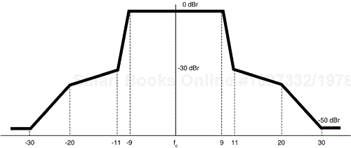
In Figure 7-9, the spectral emissions mask has been superimposed on the 11 U.S. channels. You can tell that despite having 11 channels allocated, there are actually only 3 nonover-lapping channels: 1, 6, and 11.

In the United States, CFR47 part 15.247 specifies the transmit power levels that might be used in the 2.4 GHz band. For spread spectrum systems, a 1 W peak output power with up to a 6 dBi antenna might be utilized. This combination results in a 36 dBm EIRP. For fixed-location, point-to-point links, such as what you might set up with wireless bridges, you can increase the antenna gain as long as the transmitter power is reduced by 1 dB for every 3 dB increase in antenna gain over 6 dBi. If the radio is not being used in a fixed, point-to-point application, then the transmit power must be reduced by 1 dB for every 1 dB increase in antenna gain over 6 dBi, thereby maintaining a 36 dBm EIRP limit.
For countries adopting ETSI rules, the European Telecommunications Standard (ETS) 300 328 regulation specifies the transmit power levels that may be used. It allows for a 100 mW, or 30 dBm, EIRP. In Japan, the MPT ordinance for regulating radio equipment, article 49-20 governs transmission in this band. For direct sequence spread spectrum (DSSS) signals, a 10 mW/MHz output power can be used. For frequency hopping spread spectrum (FHSS) signals, that same 10 mW/MHz can be used at frequencies from 2.471 to 2.497, but from 2.400 to 2.471 only 3 mW/MHz can be used. Israel currently follows ETSI rules for output power levels.
At press time, the U-NII band frequencies are primarily available for use in the United States and in countries that have adopted FCC-type spectrum rules. As previously stated, the U-NII 1 band extends from 5.15 to 5.25 GHz, the U-NII 2 band is immediately adjacent to it at 5.25 to 5.35 GHz, and the U-NII 3 band resides at 5.725 to 5.825 GHz. The channel numbering begins at 5.000 GHz and extends upwards from there in 5 MHz increments. This numbering provides for a channel-numbering scheme that covers the entire 5 GHz band should those frequencies ever become available for use by WLANs. Figure 7-10 shows the 8 nonoverlapping channels in the U-NII 1 and 2 bands. Note that the center frequencies for the edge channels are 30 MHz from the band edge.
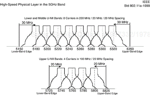
Figure 7-8 also shows the U-NII 3 channels. In contrast to the lower 5 GHz bands, the center frequencies in the U-NII 3 band are only 20 MHz from the band edge. This fact is important for you to remember when considering the spurious emissions and spectral mask requirements for this band because it proves to be more challenging for radio designers who design for the lower bands.
CFR47 part 15.407 specifies spurious emissions requirements for the three U-NII bands. For the U-NII 1 band, all emissions outside the 5.15 to 5.35 GHz band must be less than an EIRP of –27 dBm/MHz, transmissions are for indoor use only, and an integral antenna must be in use. For the U-NII 2 band, you have the option of following these same rules, although you may use the band for indoor and outdoor use with nonintegral antennas if all emissions outside of 5.25 to 5.35 are less than an EIRP of –27 dBm/MHz. For U-NII 3 band transmission, all emissions outside the band edges, 5.725 and 5.825, must be less than an EIRP of –17 dBm/MHz; furthermore, as you move to 10 MHz from the band edges, all spurious emissions must be less than or equal to an EIRP of –27 dBm/MHz.
The 802.11a standard also defines a spectral mask for transmission in the U-NII bands. The transmitted spectrum must be 0 dBr, relative to the maximum spectral density of the signal, out to a maximum bandwidth of 18 MHz, and then it must be less than –20 dBr at 11 MHz from the center frequency, -28 dBr at 20 MHz, and –40 dBr at 30 MHz. Figure 7-11 shows this spectral mask.
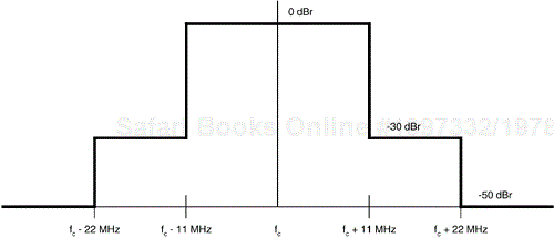
Taking your knowledge of the spectral mask and the adjacent channel rejection specified in Table 7-2, you can determine that the interfering energy contribution of an adjacent 802.11a signal while you are operating at a 6 Mbps data rate could be as high as –14 dBr, relative to your signal level, at the center frequency, as shown in Figure 7-12.

You should keep this in mind as you plan your channel allocations because contributions from multiple adjacent channels can start to accumulate.
It is also important for you to be aware of the spectral mask and spurious emissions requirements when you employ remote antennas. When vendors certify their radios and antennas with the FCC, they specifically set power levels based not only upon EIRP limits, but also upon these spectral mask constraints. It might appear that they have set antenna gains and power levels that fall below the EIRP limits, but in many cases, this setting might be necessary to meet the spectral mask requirements. For this reason, you should not exceed the vendor-suggested EIRP limits for each type of antenna and radio.
The three U-NII bands have different transmit power limitations. The U-NII 1 band is intended for indoor use only at the lowest levels. The U-NII 3 band has the highest levels because it is intended for outdoor, longer-range applications.
The following transmit power limitations are set by 802.11a for operation in the U-NII bands:
In the U-NII 1 band, you can use up to a 40 mW, 16 dBm, transmitter with up to a 6 dBi gain antenna for a 22 dBm maximum EIRP. In addition, for each dB of antenna gain over 6 dBi, you must reduce the transmitter power by 1 dB.
In the U-NII 2 band, you can use up to a 200 mW, 23 dBm, transmitter with up to a 6 dBi gain antenna for a 29 dBm maximum EIRP. In addition, for each dB of antenna gain over 6 dBi, you must reduce the transmitter power by 1 dB.
In the U-NII 3 band, you can use up to a 800 mW, 29 dBm, transmitter with up to a 6 dBi gain antenna for a 35 dBm maximum EIRP. In addition, for each dB of antenna gain over 6 dBi, you must reduce the transmitter power must be reduced by 1 dB. U-NII 3 operation allows for the use of a 23 dBi antenna without a transmitter power reduction for fixed-location, point-to-point links. This setup results in a 52 dBm maximum EIRP under these conditions.
This chapter discussed the essential physical-layer evaluation points for a radio system along with the specific rules that govern their operation. Key items to remember are that it is not enough to evaluate a radio based upon its transmit power. You must consider the entire link budget with receiver and transmitter performance characteristics. Armed with this tool, you should be able to make an informed evaluation of radios from different vendors.