

Neighborhood Processing 115
p
B
D
A
C
FIGURE 5.22: Alternative neighborhoods for a Kuwahara filter
MATLAB/Octave
>> cd = float(c);
>> cdm = imfilter(cd,ones(3)/9,’symmetric’);
>> cd2f = imfilter(cd.^2,ones(3)/9,’symmetric’);
>> cdv = cd2f - cdm.^2;
Python
In: cd = float32(c)
In: cdm = ndi.uniform
_
filter(cd,(3,3))
In: cd2f = ndi.uniform
_
filter(cd
**
2,(3,3))
In: cdv = cd2f - cdm
**
2
At this stage, the array cdm contains all the mean values, and cdv contains all the variances.
At every point (i, j) in the image then:
1. Compute the list
vars = [cdv(i − 1, j − 1), cdv( i − 1, j + 1), cdv(i + 1, j − 1), cdv(i + 1, j + 1)] .
2. Also compute the list
means = [cdm(i − 1, j − 1), cdm(i − 1, j + 1), cdm( i + 1, j − 1), cdm(i + 1, j + 1)] .
3. Output the value of “means” corresponding to the lowest value of “vars.”
Programs are given at the end of the chapter. Note that the neighborhoods can of course be
larger than 3×3, any odd square size can used, or indeed any other shape, such as shown in
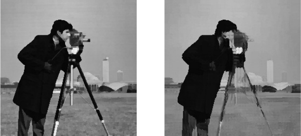
Figure 5.22. Figure 5.23 shows the cameraman image first with the Kuwahara filter using
3 ×3 neighborhoo ds and with 7 × 7 neighborhoods.
Note that even with the significant blurring with the larger filter, the edges are still
remarkably sharp.
Bilateral Filters
Linear filters (and many non-linear filters) are domain filters; the weights attached to
each neighboring pixel depend on only the position of those pixels. Another f amily of filters
are the range filters, where the weights depend on the relative difference between pixel
116 A Computational Introduction to Digital Image Processing, Second Edition
(a) Using 3 × 3 neighborhoods (b) Using 7 × 7 neighborhoods
FIGURE 5.23: Using Kuwahara filters
values. For example, consider the Gaussian filter e
(−x
2
−y
2
)/2
(so with variance σ
2
= 1) over
the region −1 ≤ x, y ≤ 1:
G =
0.36788 0.60653 0.36788
0.60653 1.00000 0.60653
0.36788 0.60653 0.36788
Applied to the neighborhood
N =
0.8 0.1 0.6
0.3 0.5 0.7
0.4 0.9 0.2
the output is simply the sum of all the pro ducts of corresponding elements of G and N.
As a range filter, however, with variance σ
2
r
, the output would be the Gaussian function
applied to the difference of the elements of N with its central value:
N − 0.5 =
0.3 −0.4 0.1
−0.2 0.0 0.2
−0.1 0.4 −0.3
For each of these values v the filter consists e
−v
2
/2σ
2
r
.
Thus, a domain filter is based on the closeness of pixels, and a range filter is based on
the similarity of pixels. Clearly, the larger the value of σ
r
the flatter the filter, and so there
will be less distinction of closeness.

Neighborhood Processing 117
The f ollowing three arrays show the results with σ
r
= 0.1, 1, 10, respectively:
σ
r
= 0.1 :
0.01111 0.00034 0.60653
0.13534 1.00000 0.13534
0.60653 0.00034 0.01111
σ
r
= 1 :
0.95600 0.92312 0.99501
0.98020 1.00000 0.98020
0.99501 0.92312 0.95600
σ
r
= 10 :
0.99955 0.99920 0.99995
0.99980 1.00000 0.99980
0.99995 0.99920 0.99955
In the last example, the values are very nearly equal, so this range filter treats all values as
being (roughly) equally similar.
The idea of the bilateral filter is to use both domain and range filtering, both with
Gaussian filters, and with variances σ
2
d
and σ
2
r
. For each pixel in the image, a range filter
is created using σ
2
r
, which maps the similarity of pixels in that neighborhood. That filter is
then convolved with the domain filter which uses σ
d
.
By adjusting the size of the filter mask, and of the variances, it is possible to obtain
varying amounts of blurring, as well as keeping the edges sharp.
At the time of writing, MATLAB’s Image Processing Toolbox does not include bilateral
filtering, but both Octave and Python do: the former with the
bilateral parameter of the
imsmooth function; the latter with the denoise
_
bilateral method in the restoration
module of skimage.
However, a simple implementation can b e written, and one is given at the chapter end.
Using any of these functions and applied to the cameraman image produces the results
shown in Figure 5.24, where in each case w gives the size of th e filter. Thus, the image in
Figure 5.24(a) can be created with our function by:
MATLAB/Octave
>> cb = bilateral(c,2,2,0,2);
where the first parameter w (in this case 2) produces filters of size 2w + 1 ×2w + 1.
Notice that even when a large flat Gaussian is used as the domain filter, as in Fig-
ure 5.24(d), the corresponding use of an appropriate range filter keeps the edges sharp.
In Python, a bilateral filter can be applied to produce, for example, the image in Fig-
ure 5.24(b) with
Python
In : import skimage.restoration as re
In : cb = re.denoise
_
bilateral(c,win
_
size=7,sigma
_
range=0.2,
...: sigma
_
spatial=10)
The following is an example of the use of Octave’s imsmooth function:
Octave
>> cb = imsmooth(c,’bilateral’,sigma
_
d=2,sigma
_
r=0.1);

118 A Computational Introduction to Digital Image Processing, Second Edition
(a) w = 5, σ
d
= 2, σ
r
= 0.2 (b) w = 7, σ
d
= 10, σ
r
= 0.2
(c) w = 11, σ
d
= 3, σ
r
= 0.1 (d) w = 11, σ
d
= 5, σ
r
= 0.5
FIGURE 5.24: Bilateral filtering

Neighborhood Processing 119
and the window size of the filter is automatically generated from the σ values.
5.10 Region of Interest Processing
Often we may not want to apply a filter to an entire image, but only to a s mall region
within it. A non-linear filter, for example, may be too computationally expensive to apply
to the entire image, or we may only be interested in the small region. Such small regions
within an image are called regions of interest or ROIs, and their processing is called region
of interest processing.
Regions of Interest in MATLAB
Before we can process a ROI, we have to define it. There are two ways: by listing the
coordinates of a polygonal region; or interactively, with the mouse. For example, suppose
we take part of a monkey image:
MATLAB/Octave
>> m2 = imread(’monkey.png’);
>> m = m2(56:281,221:412);
and attempt to isolate its head. If the image is viewed with impixelinfo, then the co-
ordinates of a hexagon that enclose the head can be determined to be ( 60, 14), (27, 38),
(14, 127), (78, 177), ( 130, 160) and (139, 69), as shown in Figure 5.25. We can then define a
region of interest using the
roipoly f unction:
MATLAB/Octave
>> xi = [60 27 14 78 130 139]
>> yi = [14 38 127 177 160 69]
>> roi=roipoly(m,yi,xi);
Note that the ROI is defined by two sets of coordinates: first the columns and then the
rows, taken in order as we traverse the ROI from vertex to vertex. In general, a ROI mask
will be a binary image the same size as the original image, with 1s for the ROI, and 0s
elsewhere. The function
roipoly can also be used interactively:
MATLAB/Octave
>> roi=roipoly(m);
This will bring up the monkey image (if it isn’t shown already). Vertices of the ROI can be
selected with the mouse: a left click selects a new vertex, backspace or delete removes the
most recently chosen vertex, and a right click finishes the selection.
Region of Interest Filtering
One of the simplest operations on a ROI is spatial filtering; this is implemented with the
function
roifilt2. With the monkey image and the ROI found above, we can experiment:
..................Content has been hidden....................
You can't read the all page of ebook, please click here login for view all page.