

Introduction 11
1.6 Image Processing Operations
It is convenient to subdivide different image processing algorithms into broad subclasses.
There are different algorithms for different tasks and problems, and often we would like to
distinguish the nature of the task at hand.
Image enhancement. This refers to processing an image so that the result is more suit-
able f or a particular application. Examples include:
• Sharpening or deblurring an out of focus image
• Highlighting edges
• Improving image contrast, or brightening an image
• Removing noise
Image restoration. This may be considered as reversing the damage done to an image
by a known cause, for example:
• Removing of blur caused by linear motion
• Removal of optical distortions
• Removing periodic interference
Image segmentation. This involves subdividing an image into constituent parts, or iso-
lating certain aspects of an image:
• Finding lines, circles, or particular shapes in an image
• In an aerial photograph, identifying cars, trees, buildings, or roads
Image registration. This involves “matching” distinct images so that they can be com-
pared, or processed together. The initial images must all be joined to share the same
coordinate system. In this text, registation as such is not covered, but some tasks
that are vital to registration are discussed, for example corner detection.
These classes are not disjoint; a given algorithm may be used for both image enhancement
or for image restoration. However, we should be able to decide what it is that we are trying
to do with our image: simply make it look better (enhancement) or removing damage
(restoration).
1.7 An Image Processing Task
We will look in some detail at a particular real-world task, and see how the above classes
may be used to describe the various stages in performing this task. The job is to obtain, by
an automatic process, the postcodes from envelopes. Here is how this may be accomplished:
Acquiring the image. First we need to produce a digital image from a paper envelope.
This can be done using either a CCD camera or a scanner.

12 A Computational Introduction to Digital Image Processing, Second Edition
Preprocessing. This is the step taken before the “major” image processing task. The
problem here is to perform some basic tasks in order to render the resulting image
more suitable for the job to follow. In this case, it may involve enhancing the contrast,
removing noise, or identifying regions likely to contain the postcode.
Segmentation. Here is where we actually “get” the postcode; in other words, we extract
from the image that part of it that contains just the postcode.
Representation and description. These terms refer to extracting the particular features
which allow us to differentiate between objects. Here we will be looking for curves,
holes, and corners, which allow us to distinguish the different digits that constitute a
postcode.
Recognition and interpretation. This means assigning labels to objects based on their
descriptors (from the previous step), and assigning meanings to those labels. So we
identify particular digits, and we interpret a string of four digits at the end of the
address as the postcode.
1.8 Types of Digital Images
We shall consider four basic types of images:
Binary. Each pixel is just black or white. Since there are only two possible values for each
pixel, we only need one bit per pixel. Such images can therefore be very efficient in
terms of storage. Images for which a binary representation may be suitable include
text (printed or handwriting), fingerprints, or architectural plans.
An example was the image shown in Figure 1.4(b). In this image, we have only the
two colors: white for the edges, and black for the background. See Figure 1.16.
1 1
0 0 0 0
0 0
1
0 0 0
0 0
1
0 0 0
0 0 0
1
0 0
0 0 0
1 1
0
0 0 0 0 0
1
FIGURE 1.16: A binary image
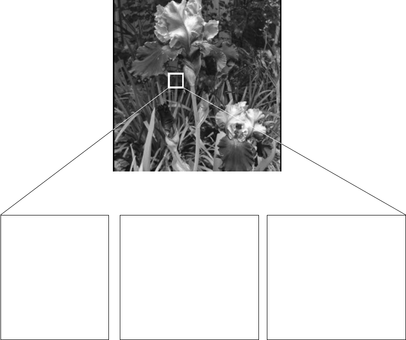
Grayscale. Each pixel is a shade of gray, normally from 0 (black) to 255 (white). This
range means that each pixel can be represented by eight bits, or exactly one byte.
This is a very natural range for image file handling. Other grayscale ranges are used,

Introduction 13
but generally they are a power of 2. Such images arise in medicine (X-rays), images
of printed works, and indeed 256 different gray levels is sufficient for the recognition
of most natural objects.
An example is the street scene shown in Figure 1.1, and in Figure 1.17.
230 229 232 234 235 232 148
237 236 236 234 233 234 152
255 255 255 251 230 236 161
99 90 67 37 94
247
130
222
152 255 129 129 246 132
154 199 255 150 189
241 147
216 132 162 163 170 239
122
FIGURE 1.17: A grayscale image
True color, or RGB. Here each pixel has a particular color; that color being described
by the amount of red, green, and blue in it. If each of these components has a range
0–255, this gives a total of 255
3
= 16,777,216 different possible colors in the image.
This is enough colors for any image. Since the total number of bits required for each
pixel is 24, such images are also called 24-bit color images.
Such an image may be considered as consisting of a “stack” of three matrices; repre-
senting the red, green, and blue values for each pixel. This means that for every pixel
there are three corresponding values.
An example is shown in Figure 1.18.
Indexed. Most color images only have a small subset of the more than sixteen million pos-
sible colors. For convenience of storage and file handling, the image has an associated
color map, or color palette, which is simply a list of all the colors used in that image.
Each pixel has a value which does not give its color (as for an RGB image), but an
index to the color in the map.
It is convenient if an image has 256 colors or less, for then the index values will only
require one byte each to store. Some image file formats (for example, Compuserve
GIF) allow only 256 colors or fewer in each image, for precisely this reason.
14 A Computational Introduction to Digital Image Processing, Second Edition
49 55 56 57 52 53
58 60 60 58 55 57
58 58 54 53 55 56
83 78
72
69 68 69
88 91 91 84 83 82
69 76 83 78 76 75
61 69 73 78 76 76
Red
64 76 82 79 78 78
93 93 91 91 86 86
88 82 88 90 88 89
125 119 113 108
111
110
137 136 132 128 126 120
105 108
114 114
118 113
96 103
112
108
111
107
Green
66 80
77
80 87
77
81 93 96 99 86 85
83 83 91 94 92 88
135 128 126
112
107 106
141
129 129
117
115 101
95 99 109 108
112
109
84 93 107 101 105 102
Blue
FIGURE 1.18: SEE COLOR INSERT A true color image

Introduction 15
Figure 1.19 shows an example. In this image the indices, rather then being the gray
values of the pixels, are simply indices into the color map. Without the color map,
the image would be very dark and colorless. In the figure, for example, pixels labelled
5 correspond to 0.2627 0.2588 0.2549, which is a dark grayish color.
4
5 5 5 5 5
5
4
5 5 6 6
5 5 5 0 8 9
5 5 5 5
11 11
5 5 5 8 16 20
8
11 11
26 33 20
11
20 33 33 58 37
Indices
0.1211 0.1211 0.1416
0.1807 0.2549 0.1729
0.2197 0.3447 0.1807
0.1611 0.1768 0.1924
0.2432 0.2471 0.1924
0.2119 0.1963 0.2002
0.2627 0.2588 0.2549
0.2197 0.2432 0.2588
Color map
FIGURE 1.19: SEE COLOR INSERT An indexed color image
1.9 Image File Sizes
Image files tend to be large. We shall investigate the amount of information used in
different image types of varying sizes. For example, suppose we consider a 512 ×512 binary
image. The number of bits used in this image (assuming no compression, and neglecting,
for the sake of discussion, any header information) is
512 ×512 × 1 = 262,144
= 32,768 bytes
= 32.768 Kb
≈ 0.033 Mb.
(Here we use the convention that a kilobyte is 1000 bytes, and a megabyte is one million
bytes.)
..................Content has been hidden....................
You can't read the all page of ebook, please click here login for view all page.