

Mathematical Morphology 291
In the right-hand grid, we have
X
0
= {p}, X
1
= {p, 1}, X
2
= {p, 1, 2}, . . .
Note that the u se of the cross-shaped structuring element means that we never cross the
boundary.
Connected Components
We use a very similar algorithm to fill a connected comp onent; we use the cross-shaped
structuring element for 4-connected components, and the square structuring element for
8-connected components. Starting with a pixel p, we fill up the rest of the component by
creating a sequence of sets
X
0
= {p}, X
1
, X
2
, . . .
such that
X
n
= (X
n−1
⊕ B) ∩A
until X
k
= X
k−1
. Figure 10.25 shows an example.
2 1 2
1
p
1
2 1 2
Using the cross
p
1 1 1
1 1
1 1 1
2
3
3
34
4 4 4
4
5
5
Using the square
FIGURE 10.25: Filling connected components
In each case, we are starting in the center of the square in the lower left. As this square is
itself a 4-connected component, the cross structuring element cannot go beyond it.
MATLAB and Octave implement this algorithm with the
bwlabel function; Python
with the
label function in the measure module of skimage. Suppose X is the image
shown in Figure 10.25. Then in MATLAB or Octave:
MATLAB/Octave
>> bwlabel(X,4)
>> bwlabel(X,8)
will show the 4-connected or 8-connected components; using the cross or square structuring
elements, respectively. In Python:
Python
In : from skimage.measure import label
In : bwlabel(X,4,background=0)+1
In : bwlabel(X,8,background=0)+1
292 A Computational Introduction to Digital Image Processing, Second Edition
The
background parameter tells Python which pixel values to treat as background; these
are assigned the value −1, all foreground components are labeled starting with the index
value 0. Adding 1 puts the background back to zero, and labels starting at 1.
MATLAB and Octave differ from Python in terms of the direction of s canning, as shown
in Figure 10.26.
[[1 1 0 2 2 0]
[1 1 1 0 2 0]
[0 0 0 2 2 2]
[3 3 3 0 0 0]
[3 3 3 0 0 0]
[3 3 3 0 0 0]]
1 1 0 3 3 0
1 1 1 0 3 0
0 0 0 3 3 3
2 2 2 0 0 0
2 2 2 0 0 0
2 2 2 0 0 0
1 1 0 1 1 0
1 1 1 0 1 0
0 0 0 1 1 1
1 1 1 0 0 0
1 1 1 0 0 0
1 1 1 0 0 0
(a) Python 4-components (b) MATLAB/Octave 4-component (c) 8-components
FIGURE 10.26: Labeling connected components
Filling holes can be done with the
bwfill function in MATLAB/Octave, or the function
binary
_
fill
_
holes
from the
ndimage
module of
scipy
:
MATLAB/Octave
>> n = imread(’nicework.png’);
>> nb = n & ~imerode(n,sq);
>> imshow(nb)
>> nf = bwfill(nb,[74,52],sq);
>> figure,imshow(nf)
Python’s command by default fills all holes by dilating and intersecting with the comple-
ment. To fill just one region:
Python
In : import skimage.morphology as mo
In : import scipy.ndimage as ndi
In : n = io.imread(’nicework.png’)/255
In : nb = n - bwerode(n,sq)
In : nb1 = nb[0:120,0:80]
In : nf = ndi.binary
_
fill
_
holes(nb1,sq)
In : nb[0:120,0:80] = nf
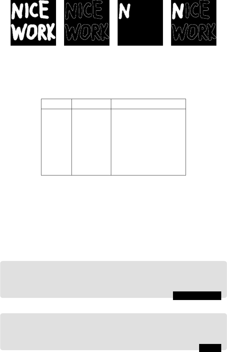
The results are shown in Figure 10.27. Image (a) is the original, (b) the boundary, and (c)
the result of a region fill. Figure (d) shows a variation on the region filling, we just include
all boundaries. This was obtained with
MATLAB/Octave
>> figure,imshow(nf|nb)
Skeletonization
Recall that the skeleton of an object can be defined by the “medial axis transform”; we
may imagine fires burning in along all edges of the object. The places where the lines of
fire meet form the skeleton. The skeleton may b e produced by morphological methods.
Mathematical Morphology 293
(a) (b) (c) (d)
FIGURE 10.27: Region filling
Consider the table of operations as shown in Table 10.1.
Erosions Openings Set differences
A A ◦B A − (A ◦ B)
A B (A B) ◦B (A B) − ((A B) ◦ B)
A 2B ( A 2B) ◦ B (A 2B) − ( ( A 2B) ◦ B)
A 3B ( A 3B) ◦ B (A 3B) − ( ( A 3B) ◦ B)
.
.
.
.
.
.
.
.
.
A kB (A kB) ◦ B (A kB) − ((A kB) ◦ B)
TABLE 10.1: Operations used to construct the skeleton
Here we use the convention that a sequence of k erosions using the same structuring
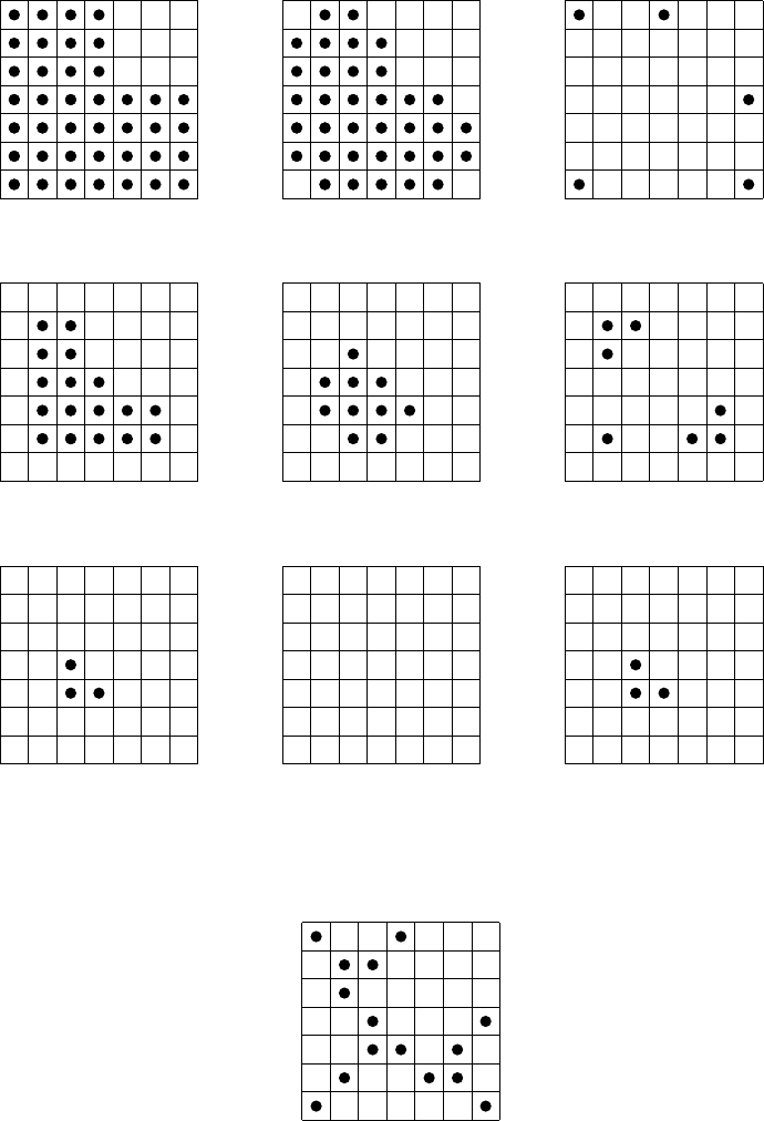
element B is denoted A kB. We continue the table until (A kB) ◦ B is empty. The
skeleton is then obtained by taking the unions of all the set differences. An example is given
in Figure 10.28, using the cross-shaped structuring element.
Since (A 2B) ◦ B is empty, we stop here. The skeleton is the union of all the sets
in the third column; it is shown in Figure 10.29. This method of skeletonization is called
Lantuéjoul’s method; for details, see Serra [45].
Programs are given at the end of the chapter. We shall experiment with the nice work
image, either with MATLAB or Octave:
MATLAB/Octave
>> nk = imskel(n,sq);
>> imshow(nk)
>> nk2 = imskel(n,cr);
>> figure,imshow(nk2)
or with Python:
Python
In : nk = bwskel(n,sq)
In : io.imshow(nk)
In : nk2 = bwskel(n,cr)
In : f = plt.figure(); f.show(io.imshow(nk2))
294 A Computational Introduction to Digital Image Processing, Second Edition
A A ◦ B
A −(A ◦ B)
A B
(A B) ◦B (A B) − ((A B) ◦ B)
A 2B
(A 2B) ◦B (A 2B) − ((A 2B) ◦ B)
FIGURE 10.28: Skeletonization
FIGURE 10.29: The final skeleton
Mathematical Morphology 295
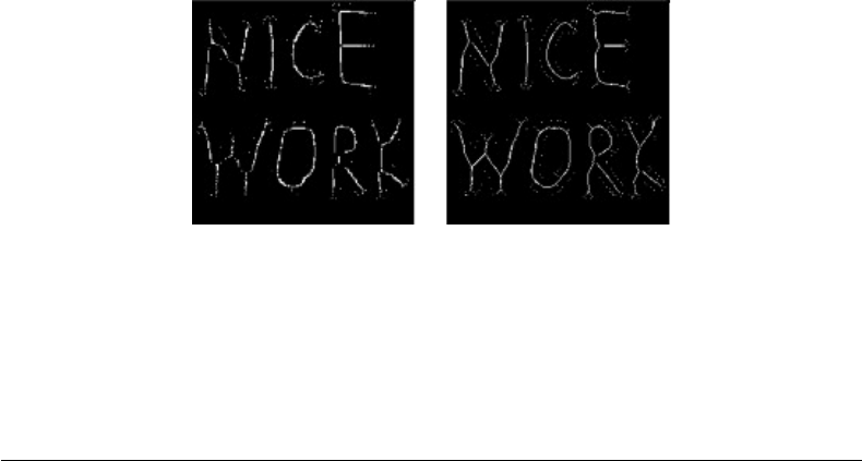
The results are shown in Figure 10.30. Image (a) is the result using the square structuring
element; image (b) is the result using the cross structuring element.
(a) (b)
FIGURE 10.30: Skeletonization of a binary image
10.7 A Note on the bwmorph Function in MATLAB and Octave
The theory of morphology developed so far uses versions of erosion and dilation some-
times called generalized erosion and dilation; so called because the definitions allow for
general structuring elements. This is the method used in the
imerode and imdilate func-
tions. However, the
bwmorph function actually uses a different approach to morphology;
that based on lookup tables. (Note however that Octave’s
bwmorph function implements
erosion and dilation with calls to the
imerode and imdilate functions.) We have seen the
use of lookup tables for binary operations in Chapter 11; they can be just as easily applied
to implement morphological algorithms.
The idea is simple. Consider the 3 × 3 neighborhood of a pixel. Since each pixel in the
neighborhood can only have two values, there are 2
9
= 512 different possible neighborhoods.
We define a morphological operation to be a function that maps these neighborhoods to the
values 0 and 1. Each possible neighborhood state can be associated with a numeric value
from 0 (all pixels have value 0) to 511 (all pixels have value 1). The lookup table is then a
binary vector of length 512; its k-th element is the value of the function for state k.
With this approach, we can define dilation as follows: a 0-valued pixel is changed to
1 if at least one of its eight neighbors has value 1. Conversely, we may define erosion as
changing a 1-valued pixel to 0 if at least one of its eight neighbors has value 0.
Many other operations can be defined by this method (see the help file for
bwmorph). The
advantage is that any operation can be implemented extremely easily, simply by listing the
lookup table. Moreover, the use of a lookup table allows us to satisfy certain requirements;
the skeleton, for example, can be connected and have exactly one pixel thickness. This is
not necessarily true of the algorithm presented in Section 10.6. The disadvantage of lookup
tables is that we are restricted to using 3 × 3 neighborhoods. For more details, see “Digital
Image Processing” by W. K. Pratt [35].
..................Content has been hidden....................
You can't read the all page of ebook, please click here login for view all page.