

366 A Computational Introduction to Digital Image Processing, Second Edition
This means that when we exclude elements from the transform, they must be excluded in
pairs. In other words, given a transform with N elements, all but 2k + 1 elements can be
excluded as shown in Figure 12.10.
DC
k elements
N − 2k − 1 zeros
k elements
FIGURE 12.10: Excluding elements from the DFT
In order to approximate a shape, given 2k + 1 non-zero elements of a transform, there
are several possibilities:
1. Apply the inverse transform to the complete N length vector (including the zeros),
and plot the result.
2. Simply invert the smaller vector of 2k + 1 elements, and plot those values joined by
lines.
3. Place any number of zeros between the first k + 1 and last k values b ef ore inversion.
Consider a large shape with many boundary pixels:
MATLAB/Octave
>> z = zeros(256);
>> z(32:224,32:96) = 1; z(32:96,96:224) = 1; z(192:224,96:160) = 1;
>> [cc,bdy] = shape(z,4)
There are 896 pixels in the boundary. Now to transform them and delete most of them,
first in MATLAB or Octave:
MATLAB/Octave
>> c = complex(bdy(:,1),bdy(:,2));
>> N = length(c)
N = 896
>> cf = fft(c);
>> k = 12;
>> cf2 = cf; cf2(k+2:N-k) = 0;
>> bdy2 = ifft(cf2);
>> cf3 = [cf(1:k+1);cf(N-k+1:N)];
>> bdy3 = ifft(cf3);
>> cf4 = [cf3(1:13);zeros(100,1);cf3(14:25)];
>> bdy4 = ifft(cf4);
or in Python:

Shapes and Boundaries 367
Python
In : from numpy.fft import fft, ifft
In : execfile(’chaincode.py’)
In : z = np.zeros((256,256))
In : z[31:224,31:96] = 1;z[31:96,95:223] = 1; z[192:224,95:160]=1
In : cc,bdy = shape(z)
In : c = bdy[:,0]+bdy[:,1]
*
1j
In : k = 12; N = len(c)
In : cf = fft(c); cf2 = np.copy(cf); cf2[k+1:N-k]=0; bdy2 = ifft(cf2);
In : cf3 = np.hstack((cf[:k+1],cf[-k:])); bdy3 = ifft(cf3)
In : cf4 = np.hstack((cf[:k+1],np.zeros((100)),cf[-k:])); bdy4 = ifft(cf4)
At this stage cf2 consists of 896 values, most of them zero, and so bdy2 has 896 values.
But
cf3
consists only of the first 13 and last 12 values of
cf
—in effect
cf3
is
cf2
with all
the zero elements removed—and so both it and
bdy3
have only 25 values. Finally,
cf4
is
created from
cf3 by putting in 100 zeros between the first k + 1 and final k values. There
is nothing special about 100—any value will do—but the larger the value, the more points
will fill out the boundary.
So the plots can be created as
MATLAB/Octave
>> plot(bdy2,’.’),axis([0,256,0,256]),axis equal,axis nolabel
>> plot([bdy3;bdy3(1)],’.-’,"markersize",5),axis([0,10000,0,10000]),...
axis equal,axis nolabel
>> plot(bdy4,’.’),axis([0 2000 0 2000]),axis equal,axis nolabel
or as
Python
In : plt.plot(bdy2.real,bdy2.imag,’.’); plt.axis(’equal’)
In : bdy3 = np.hstack(bdy3,bdy3[0])
In : plt.plot(bdy3.real,bdy3.imag,’.-’,markersize=5); plt.axis
([0,9000,0,9000])
In : plt.plot(bdy4.real,bdy4.imag,’.’); plt.axis([0.0,2000.0,0.0,2000.0])
and the results are shown in Figure 12.11.
bdy2: 896 points bdy3: 25 points joined with lines bdy4: 25 + 100 points
FIGURE 12.11: Fourier descriptors drawn differently
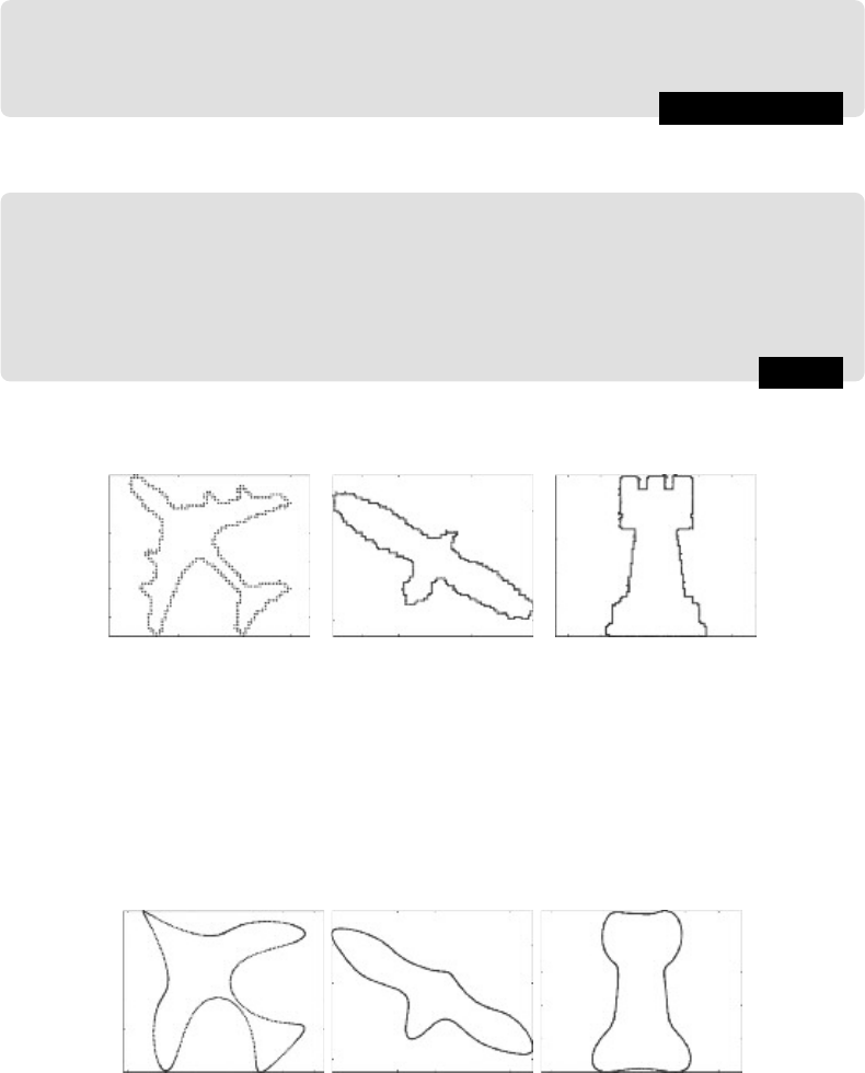
To give a slightly more substantial example, consider the three shapes in Figure 12.12.
Each one can be plotted from a list of points; for example, the plane can be created in
MATLAB or Octave with:
368 A Computational Introduction to Digital Image Processing, Second Edition
MATLAB/Octave
>> pl = dlmread(’plane.txt’);
>> c = complex(pl(:,1),pl(:,2));
>>
plot
(c,’.’),axis equal, axis nolabel
or in Python with
Python
In : pl = np.loadtxt(’plane.txt’)
In : c = pl[:,0] + pl[:,1]
*
1j
In : plt.plt.plot(c.real,c.imag,’.’)
In : plt.axis(’equal’)
In : plt.tick
_
params(axis=’both’,labelbottom=’off’,labelleft=’off’)
In : plt.show()
where the plt.tick
_
params function turns off the tick marks on the axes. Each of the
plane.txt eagle.txt chess.txt
FIGURE 12.12: Three shapes
three shapes has roughly the same number of boundary points: between 415 and 420.
For each of the values k = 8, 20, 32 set all but the first k + 1 and last k of the transform
values to zero, and invert the result. So Figure 12.13 shows the Fourier descriptors with
k = 8. Although the boundaries are quite blurred, and fine details are missing, the basic
FIGURE 12.13: Using only 8 pairs of values from the Fourier transform
nature of the shapes, and their sizes and orientations are quite clear.
So Figure 12.14 shows the Fourier descriptors with k = 20. With more values used some
fine detail begins to appear: the engines on the plane wings and the detail on the top of
the chess piece. Even more detail is apparent with k = 32, as shown in Figure 12.15.
Although the b oundaries are still not as sharp as the originals, a remarkable amount of
detail is apparent for only 32 of the roughly 210 pairs of values in the transf orm.

Shapes and Boundaries 369
FIGURE 12.14: Using 20 pairs of values from the Fourier transform
FIGURE 12.15: Using 32 pairs of values from the Fourier transform
Exercises
1. Find the chain codes, normalized chain codes, and shape numbers for each of the
4-connected shapes given in Figure 12.16.
2. Now repeat the above exercise for all possible reflections and rotations of those shapes.
3. Repeat the above exercises for the 8-connected shapes given in Figure 12.17.
4. Check your answers to the previous questions with the
shape program.
5. Generate the shapes with the following 4-connected chain codes:
(a)
3 3 3 0 0 0 0 1 1 2 2 1 2 2
(b) 3 3 3 0 3 0 0 1 0 1 1 2 2 1 2 2
6. Generate the shapes with the following 8-connected chain codes:
(a)
5 6 7 6 0 0 1 2 2 4 3 4
FIGURE 12.16: Shapes for Question 1

370 A Computational Introduction to Digital Image Processing, Second Edition
FIGURE 12.17: Shapes for Question 3
(b)
5 6 7 7 1 7 1 2 2 3 5 3 4
7. Obtain the normalized chaincodes and shape numbers of all the shapes in the previous
questions.
Check your answers with
shape.
8. Use your system to generate a T shape, and obtain its Fourier descriptors. How many
terms are required to identify the
(a) Symmetry of the object?
(b) Size of the object?
(c) Shape of the object?
9. Repeat the above question but use an X shape. Then again, but with an E shape.
10. Compare the results of the shapes in the previous two questions. How many terms
are required to distinguish the
(a) Symmetries
(b) Sizes
(c) Shapes
of the three objects?
11. How does the size of an object affect its Fourier descriptors? Experiment with a 6 ×4
rectangle, and then with a 12 × 8 rectangle. Generalize your findings.
..................Content has been hidden....................
You can't read the all page of ebook, please click here login for view all page.