

130 A Computational Introduction to Digital Image Processing, Second Edition
MATLAB/Octave
>> c = imread(’cameraman.png’);
>> head = c(33:96,90:153);
>> imshow(head)
>> head4n = imresize(head,4,’nearest’);imshow(head4n)
>> head4b = imresize(head,4,’bilinear’);imshow(head4b)
Python has a rescale function in the transform module of skimage:
Python
In : c = io.imread(’cameraman.png’)
In : head = c[32:96,89:153]
In : io.imshow(head)
In : head4n = tr.rescale(head,2,order=0)
In : head4n = tr.rescale(head,2,order=1)
The order parameter of the rescale method provides the order of the interpolating p oly-
nomial: 0 corresponds to nearest neighbor and 1 to bilinear interpolation.
The head is shown in Figure 6.8 and the results of the scaling are shown in Figure 6.9.
FIGURE 6.8: The head
Nearest neighbor interpolation gives an unacceptable blo cky effect; edges in particular
appear very jagged. Bilinear interpolation is much smoother, but the trade-off here is a
certain blurriness to the result. This is unavoidable: interpolation can’t predict values: we
can’t create data from nothing! All we can do is to guess at values that fit b est with the
original data.
6.3 General Interpolation
Although we have presented nearest neighbor and bilinear interpolation as two different
methods, they are in fact two special cases of a more general approach. The idea is this:
we wish to interpolate a value f(x
) for x
1
≤ x
≤ x
2
, and suppose x
− x
1
= λ. We define
an interpolation function R(u), and set
f(x
) = R (− λ ) f (x
1
) + R(1 − λ)f(x
2
). (6.2)

Image Geometry 131
(a) Nearest neighbor scaling (b) Bilinear interpolation
FIGURE 6.9: Scaling by interpolation
Figure 6.10 shows how this works. The function R(u) is centered at x
, so x
1
corresponds
x
1
x
x
2
R(−λ)
R(1 − λ)
R(0)
FIGURE 6.10: Using a general interpolation function
with u = −λ, and x
2
with u = 1 − λ. Now consider the two functions R
0
(u) and R
1
(u)
shown in Figure 6.11. Both these functions are defined on the interval −1 ≤ u ≤ 1 only.
Their f ormal definitions are:
−1 −0.5 0 0.5 1
R
0
(u)
−1 0 1
R
1
(u)
FIGURE 6.11: Two interpolation functions

132 A Computational Introduction to Digital Image Processing, Second Edition
R
0
(u) =
0 if u ≤ −0.5
1 if −0.5 < u ≤ 0.5
0 if u > 0.5
and
R
1
(u) =
1 + u if u ≤ 0
1 −u if u ≥ 0
The function R
1
(u) can also be written as 1 − |x|. Now substituting R
0
(u) f or R(u) in
Equation 6.2 will produce nearest neighbor interpolation. To see this, consider the two
cases λ < 0.5 and λ ≥ 0.5 separately. If λ < 0.5, then R
0
(−λ) = 1 and R
0
(1 −λ) = 0. Then
f(x
) = (1)f (x
1
) + (0)f (x
2
) = f (x
1
).
If λ ≥ 0.5, then R
0
(−λ) = 0 and R
0
(1 −λ) = 1. Then
f(x
) = (0)f (x
1
) + (1)f (x
2
) = f (x
2
).
In each case f(x
) is set to the function value of the point closest to x
.
Similarly, substituting R
1
(u) for R(u) in Equation 6.2 will produce linear interpolation.
We have
f(x
) = R
1
(−λ)f(x
1
) + R
1
(1 −λ)f (x
2
)
= (1 − λ) f (x
1
) + λf(x
2
)
which is the correct equation.
The functions R
0
(u) and R
1
(u) are just two members of a family of possible interpolation
functions. Another such function provides cubic interpolation; its definition is:
R
3
(u) =
1.5|u|
3
− 2.5|u|
2
+ 1 if | u| ≤ 1,
−0.5|u|
3
+ 2.5|u|
2
− 4|u|+ 2 if 1 < |u| ≤ 2.
Its graph is shown in Figure 6.12. This function is defined over the interval −2 ≤ u ≤ 2,
−2 −1 0 1 2
FIGURE 6.12: The cubic interpolation function R
3
(u)
and its use is slightly different from that of R
0
(u) and R
1
(u), in that as well as using the
function values f(x
1
) and f(x
2
) for x
1
and x
2
on either side of x
, we use values of x further
away. In fact the formula we use, which extends Equation 6.2, is:
f(x
) = R
3
(−1 −λ)f (x
1
) + R
3
(−λ)f(x
2
) + R
3
(1 −λ)f (x
3
) + R
4
(2 −λ)f (x
4
)
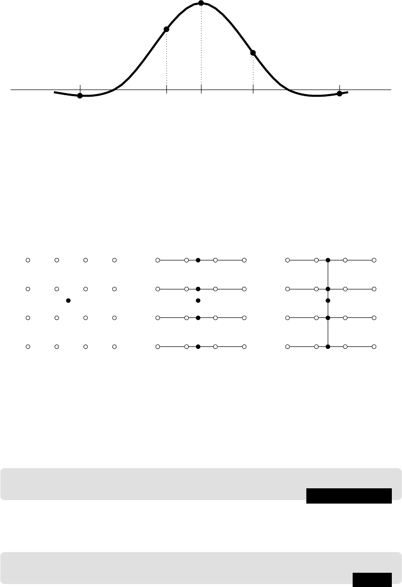
Image Geometry 133
x
1
x
2
x
x
3
x
4
R
3
(−1 −λ)
R
3
(−λ)
R
3
(0)
R
3
(1 −λ)
R
3
(2 −λ)
FIGURE 6.13: Using R
3
(u) for interpolation
where x
is between x
2
and x
3
, and x − x
2
= λ. Figure 6.13 illustrates this. To apply
this interpolation to images, we use the 16 known values around our p oint (x
, y
). As
for bilinear interpolation, we first interpolate along the rows, and then finally down the
columns, as shown in Figure 6.14. Alternately, we could first interpolate down the columns,
and then across the row. This means of image interpolation by applying cubic interpolation
in both directions is called bicubic interpolation. To perform bicubic interpolation on an
Initial points Interpolating along
rows
Interpolating down
the column
FIGURE 6.14: How to apply bicubic interpolation
image with MATLAB, we use the
’bicubic’ method of the imresize function. To enlarge
the cameraman’s head, we enter (for MATLAB or Octave):
MATLAB/Octave
>> head4c = imresize(head,4,’bicubic’);imshow(head4c)
In Python the order parameter of rescale must be set to 3 for bicubic interpolation:
Python
In : head4c = tr.rescale(head,4,order=3)
and the result is shown in Figure 6.15.

134 A Computational Introduction to Digital Image Processing, Second Edition
FIGURE 6.15: Enlargement using bicubic interpolation
6.4 Enlargement by Spatial Filtering
If we merely wish to enlarge an image by a power of 2, there is a quick and dirty method
which uses linear filtering. We give an example. Suppose we take a simple 4 × 4 matrix:
MATLAB/Octave
>> m = magic(4)
m =
16 2 3 13
5 11 10 8
9 7 6 12
4 14 15 1
Our first step is to create a zero-interleaved version of this matrix. This is obtained by
interleaving rows and columns of zeros between the rows and columns of the original matrix.
Such a matrix will be double the size of the original, and will contain mostly zeros. If m
2
is the zero-interleaved version of m, then it is defined by:
m
2
(i, j) =
m((i + 1)/2, (j + 1)/2) if i and j are both odd,
0 otherwise.
This can be implemented very simply:
..................Content has been hidden....................
You can't read the all page of ebook, please click here login for view all page.