

Wavelets 441
f(x, y)
Original image
1-scale DWT 2-scale DWT 3-scale DWT
FIGURE 15.5: The non-standard decomposition of the two-dimensional DWT
15.3 Wavelets and Images
Each of MATLAB, Octave, and Python has some wavelet functionality, either built in
or available through an added toolbox or package. However, the standard packages all seem
to work a little differently. Happily for us, there is an open-source wavelet package with
bindings f or each of MATLAB, Octave, and Python f rom Rice University, obtainable from
http://dsp.rice.edu/software/rice-wavelet-toolbox
Assuming that the toolbox has been downloaded and installed, we can try it, using the
same vector as above:
MATLAB/Octave
>> [h,g] = daubcqf(2)
h =
0.70711 0.70711
g =
-0.70711 0.70711
Here h and g are the low pass and high pass filter coefficients for the forward transform. The
daubcqf function produces the filter coefficients for a class of wavelets called Daubechies
wavelets, of which the Haar wavelet is the simplest. Now we can apply the DWT to our
vector:
MATLAB/Octave
>> format bank
>> w = mdwt(v,h,1)
w =
97.58 35.36 48.08 22.63 2.83 -1.41 2.83 -2.83
This is not quite the same as the first vector W from above, but is off only by a single
scaling f actor:
MATLAB/Octave
>> w
*
sqrt(2)
ans =
138.00 50.00 68.00 32.00 4.00 -2.00 4.00 -4.00

442 A Computational Introduction to Digital Image Processing, Second Edition
which is the same result we obtained earlier by adding and subtracting. The transforms at
2 and 3 scales can be given simply by adjusting the final parameter:
MATLAB/Octave
>> w2 = mdwt(v,h,2)
w2 =
94.00 50.00 44.00 18.00 2.83 -1.41 2.83 -2.83
>> w3 = mdwt(v,h,3)
w3 =
101.82 31.11 44.00 18.00 2.83 -1.41 2.83 -2.83
To go backward, use the inverse transform:
MATLAB/Octave
>> format
>> midwt(w3,h,3)
ans =
71.000 67.000 24.000 26.000 36.000 32.000 14.000 18.000
Note that we can supply our own filter values:
MATLAB/Octave
>> h = [1 1]
>> mdwt(v,h,1)
ans =
138 50 68 32 4 -2 4 -4
>> mdwt(v,h,2)
ans =
188 100 88 36 4 -2 4 -4
>> mdwt(v,h,3)
ans =
288 88 88 36 4 -2 4 -4
and these are indeed the values we obtained earlier simply by adding and subtracting.
The Python equivalent commands require the loading of the
rwt library. Then:

Wavelets 443
Python
In : h,g = rwt.daubcqf(2)
In : print rwt.dwt(v,h,1)[0]
[ 97.5807 35.3553 48.0833 22.6274 2.8284 -1.4142 2.8284 -2.8284]
In : print rwt.dwt(v,h,3)[0]
[ 101.8234 31.1127 44. 18. 2.8284 -1.4142 2.8284 -2.8284]
In : h = np.array([1,1]).astype(’float’)
In : vw = rwt.dwt(v,h,3)[0]
In : print vw[0]
[ 288. 88. 88. 36. 4. -2. 4. -4.]
In : hi = np.array([0.5,0.5]).astype(’float’)
In : print rwt.idwt(vw[0],hi,3)[0]
[ 71. 67. 24. 26. 36. 32. 14. 18.]
Let’s try an image. We shall apply the Haar wavelet to an image of size 256 × 256, first at
one scale. For display, it will be necessary to scale parts of the image for viewing.
MATLAB/Octave
>> c = imread(’cameraman.png’);
>> h = daubcqf(2)
>> cw1 = mdwt(double(c),h,1);
Now at this stage some adjustment needs to be done to display the transform. Because the
range of values in the transform
cw1 is large:
MATLAB/Octave
>> [max(cw1(:)),min(cw1(:))]
ans =
501.00 -209.50
some method will be needed to adjust those values for display. In MATLAB or Octave,
since
cw1 is an array of data type double, elements outside the range 0.0 − −1.0 will be
displayed as black or white. Adjustment can be done in several ways; first by simply using
mat2gray, second by a log function, as was done for the Fourier transform:
MATLAB/Octave
>> imshow(cw1)
>> figure, imshow(mat2gray(cw1))
>> cwlog = log(1+abs(cw1))
>> figure, imshow(mat2gray(cwlog))
In Python, this is more easily done as images are automatically scaled for display:
Python
In : h,g = rwt.daubcqf(2)
In : cw1 = rwt.dwt(castype(’float’),h,1)[0]
In : cwlog = np.log(1+abs(cw1))
and both cw1 and cwlog can be displayed simply with io.imshow. All three images are
shown in Figure 15.6. Now consider the same transform, but at 3 scales:
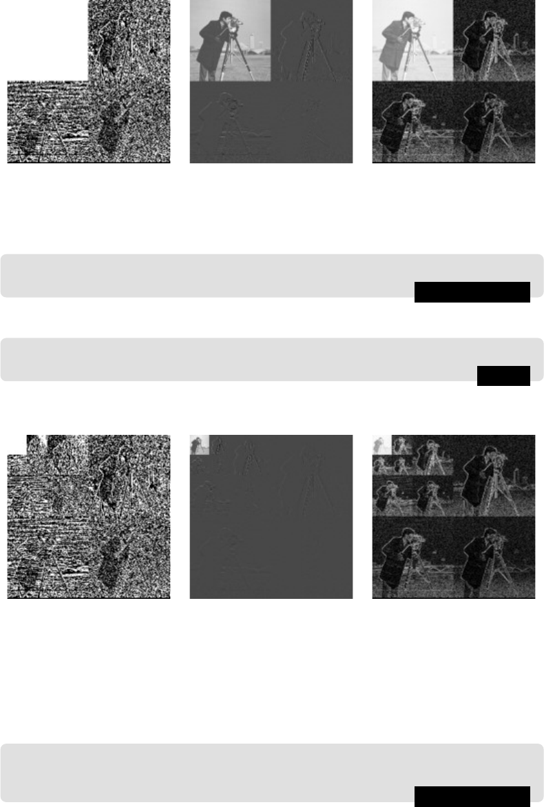
444 A Computational Introduction to Digital Image Processing, Second Edition
(a) No adjustment (b) With
mat2gray
(c) With log and
mat2gray
FIGURE 15.6: Different displays of a 1-scale DWT applied to an image
MATLAB/Octave
>> cw3 = mdwt(double(c),h,3);
or with
Python
In : cw1 = rwt.dwt(castype(’float’),h,3)[0]
and the result with the same adjustments as above is shown in Figure 15.7.
(a) No adjustment (b) With mat2gray (c) With log and mat2gray
FIGURE 15.7: Different displays of a 3-scale DWT applied to an image
This wavelet transform can be seen to use the non-standard decomposition. To see what
a standard decomposition looks like, we can multiply the rows, and then the columns, by
the appropriate Haar matrix:
MATLAB/Octave
>> H = [1 1;1 -1];
>> for i = 1:2, H = [kron(H,[1 1]);kron(eye(size(H)),[1,-1])]; end
or in Python as

Wavelets 445
Python
In : H = np.array([[1,1],[1,-1]])
In : for i in range(2):
...: H = np.vstack([np.kron(H,[1,1]),np.kron(np.eye(H.shape[0]),[1,-1])
])
...:
So far this is the 3-scale 8 × 8 matrix, which now needs to be scaled up to be 256 × 256:
MATLAB/Octave
>> K1 = kron(eye(32),H(1,:));
>> K2 = kron(eye(32),H(2,:));
>> K3 = kron(eye(32),H(3:4,:));
>> K4 = kron(eye(32),H(5:8,:));
>> H = [K1;K2;K3;K4];
or
Python
In : K1 = np.kron(np.eye(32),H[0,:])
In : K2 = np.kron(np.eye(32),H[1,:])
In : K3 = np.kron(np.eye(32),H[2:4,:])
In : K4 = np.kron(np.eye(32),H[4:8,:])
In : H = np.vstack([K1,K2,K3,K4])
The next step is to scale the rows so that the matrix is orthogonal:
MATLAB/Octave
>> D = diag(diag(H
*
H’));
>> H = sqrt(inv(D))
*
H;
or
Python
In : D = H.dot(H.T)
In : np.sqrt(np.linalg.inv(D)).dot(H)
This last H is the matrix we want, which implements a Haar 3-scale wavelet transform on
vectors of length 256. It can be applied to the image:
MATLAB/Octave
>> cw = (H
*
(H
*
double(c))’)’;
or with
Python
In : cw = H.dot(H.dot(c.astype(’float’)).T).T
and displayed with the log scaling, as shown in Figure 15.8. With the log scaling, it is
clear that in the standard decomposition, the filtered images in the transform are squashed,
rather than all retaining their shape as in the non-standard decomposition.
..................Content has been hidden....................
You can't read the all page of ebook, please click here login for view all page.