
228 A Computational Introduction to Digital Image Processing, Second Edition
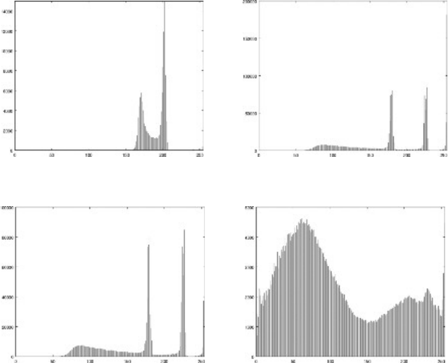
Blood smear image:
blood.png
Paramecium image:
paramecium1.png
Pine nuts image: pinenuts.png Daisies image: daisies.png
FIGURE 9.6: Histograms
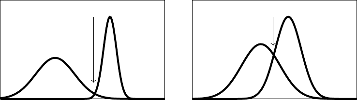
Image Segmentation 229
The trouble is that in general the individual histograms of the objects and background
will overlap, and without prior knowledge of the individual histograms it may be difficult to
find a splitting point. Figure 9.7 illustrates this, assuming in each case that the histograms
for the objects and backgrounds are those of a normal distribution. Then we choose the
Threshold Threshold
FIGURE 9.7: Splitting up a histogram for thresholding
threshold values to be the place where the two histograms cross over.
In practice though, the histograms won’t be as clearly defined as those in Figure 9.7, so
we need some sort of automatic method for choosing a “best” threshold. There are in fact
many different methods; here are two.
Otsu’s Method
This was first described by Nobuyuki Otsu in 1979. It finds the best place to threshold
the image into “foreground” and “background” components so that the inter-class variance—
also known as the between class variance—is maximized. Suppose the image is divided into
foreground and background pixels at a threshold t, and the fractions of each are w
f
and w
b
respectively. Suppose also that the means are µ
f
and µ
b
. Then the inter-class variance is
defined as
w
f
w
b
(µ
f
− µ
b
)
2
.
If an image has n
i
pixels of gray value i, then define p
i
= n
i
/N where N is the total number
of pixels. Thus, p
i
is the probability of a pixel having gray value i. Given a threshold value
t then
w
b
=
t−1
k=0
p
k
,
w
f
=
L−1
k=t
p
k
.
where L is the number of gray values in the image. S ince by definition we must have
L−1
k=0
p
k
= 1
it follows that w
k
+ w
f
= 1. The background weights can be computed by a cumulative
sum of all the p
k
values.

230 A Computational Introduction to Digital Image Processing, Second Edition
The means can be defined as
µ
b
=
1
w
b
t−1
k=0
kp
k
,
µ
f
=
1
w
f
L−1
k=t
kp
k
.
Note that the sums
t−1
k=0
kp
k
again can be computed by cumulative sums, and
L−1
k=t
kp
k
=
L−1
k=0
kp
k
−
t−1
k=0
kp
k
.
and the first term on the left is fixed.
For a simple example, consider an 8 ×8 3-bit image with the following values of n
k
and
p
k
= n
k
/N = n
k
/64
i n
i
p
i
0 4 0.062500
1 8 0.125000
2 10 0.156250
3 9 0.140625
4 4 0.062500
5 8 0.125000
6 12 0.187500
7 9 0.140625
Then the other values can be computed easily:
k n
k
p
k
w
b
w
f
kp
k
kp
k
µ
b
µ
f
vars
0 4 0.06250 0.06250 0. 93750 0.00000 0.00000 0.00000 4.10000 0.98496
1 8 0.12500 0.18750 0. 81250 0.12500 0.12500 0.66667 4.57692 2.32935
2 10 0.15625 0.34375 0.65625 0.31250 0.43750 1.27273 5.19048 3.46246
3 9 0.14062 0.48438 0. 51562 0.42188 0.85938 1.77419 5.78788 4.02348
4 4 0.06250 0.54688 0. 45312 0.25000 1.10938 2.02857 6.03448 3.97657
5 8 0.12500 0.67188 0. 32812 0.62500 1.73438 2.58140 6.42857 3.26296
6 12 0.18750 0.85938 0.14062 1.12500 2.85938 3.32727 7.00000 1.63013
7 9 0.14062 1.00000 0. 00000 0.98438 3.84375 3.84375 − −
So in this case, we have
µ
f
=
1
w
f
3.84375 −
t−1
k=0
kp
k
.
The largest value of the inter-class variance is at k = 3, which means that t −1 = 3 or t = 4
is the optimum threshold.
And in fact if a histogram is drawn as shown in Figure 9.8 it can b e seen that this is a
reasonable place for a threshold.

Image Segmentation 231
0 1 2 3 4 5 6 7
2
4
6
8
10
12
FIGURE 9.8: An example of a histogram illustrating Otsu’s method
The ISODATA Method
ISODATA is an acronym for “Iterative Self-Organizing Data Analysis Technique A,”
where the final “A” was added, according to the original paper, “. . . to make ISODATA
pronouncable.” It is in fact a very simple method, and in practice converges very fast:
1. Pick a precision value and a starting threshold value t. Often t = L/2 is used.
2. Compute µ
f
and µ
b
for this threshold value.
3. Compute t
= (µ
b
+ µ
f
)/2.
4. If | t − t
| < the stop and return t, else put t = t
and go back to step 2.
On the cameraman image
c, for example, the means can be quickly set up in MATLAB and
Octave using the
cumsum function, which produces the cumulative sum of a one-dimensional
array, or of the columns of a two-dimensional array:
MATLAB/Octave
>> k = (0:255)’;
>> n = histc(c(:),k); p = n/prod(size(c));
>> wb = cumsum(p); wf = 1-wb;
>> kpc = cumsum(k.
*
p);
>> mu
_
b = kpc./wb; mu
_
f = (kpc(end)-kpc)./wf;
and in Python also using its cumsum function:
Python
In : k = np.arange(256)
In : n = ndi.histogram(c,0,255,256); p = n/(c.size+0.0)
In : wb = np.cumsum(p); wf = 1-wb
In : kpc = np.cumsum(k
*
p)
In : mu
_
b = kpc/wb; mu
_
f = (kpc[-1]-kpc)/wf;
Now to compute 10 iterations of the algorithm (this saves having to set up a stopping
criterion with a precision value):

232 A Computational Introduction to Digital Image Processing, Second Edition
MATLAB/Octave
>> t = 128
>> for i = 1:10,
> t1 =
floor
((mu
_
b(t)+mu
_
f(t))/2),
> t = t1;
> end
t1 = 108
t1 = 95
t1 = 89
t1 = 88
t1 = 88
t1 = 88
t1 = 88
t1 = 88
t1 = 88
t1 = 88
Python
In : t = 128
In : for i in range(10):
...: t1 = int((mu
_
f[t]+mu
_
b[t])/2.0)
...: print t1
...: t = t1
...:
108
95
90
88
88
88
88
88
88
88
The iteration quickly converges in only four steps.
MATLAB and Octave provide automatic thresholding with the graythresh function,
with parameters
’otsu’ and ’intermeans’ in Octave for Otsu’s method and the ISODATA
method. In Python there are the methods
threshold
_
otsu and threshold
_
isodata in
the
filter module of skimage.
Consider four images,
blood.png, paramecium1.png, pinenuts.png, and daisies.png
which are shown in Figure 9.9.
With the images saved as arrays
b, p, n, and d, the threshold values can be computed
in Octave as follows, by setting up an anonymous function to perform thresholding:
Octave
>> thresh = @(x) [graythresh(x,’otsu’),graythresh(x,’intermeans’)];
>> ts = cellfun(@thresh, {b,p,n,d},’UniformOutput’,false);
>> for i = 1:4, disp(ts{i}), end
0.74510 0.74510
0.75294 0.75294
0.47451 0.47451
0.51373 0.51373
..................Content has been hidden....................
You can't read the all page of ebook, please click here login for view all page.