

Chapter 6
Image Geometry
There are many situations in which we might want to change the shape, size, or orientation
of an image. We may wish to enlarge an image, to fit into a particular space, or f or printing;
we may wish also to reduce its size, say for inclusion on a web page. We might also wish to
rotate it: maybe to adjust for an incorrect camera angle, or simply f or affect. Rotation and
scaling are examples of affine transformations, where lines are transformed to lines, and
in particular parallel lines remain parallel after the transformation. Non-affine geometrical
transformations include warping, which we will not consider.
6.1 Interpolation of Data
We will start with a simple problem: suppose we have a collection of 4 values, which
we wish to enlarge to 8. How do we do this? To start, we have our points x
1
, x
2
, x
3
, and
x
4
, which we su ppose to be evenly spaced, and we have the values at those points: f (x
1
),
f(x
2
), f(x
3
), and f (x
4
). Along the line x
1
. . . x
4
we wish to space eight points x
1
, x
2
, . . . , x
8
.
Figure 6.1 shows how this would be done.
x
1
x
2
x
3
x
4
x
1
x
2
x
3
x
4
x
5
x
6
x
7
x
8
FIGURE 6.1: Replacing four points with eight
Suppose that the distance between each of the x
i
points is 1; thus, the length of the line
is 3. Thus, since there are seven increments from x
i
to x
8
, the distance between each two
will be 3/7 ≈ 0.4286. To obtain a relationship between x and x
we draw Figure 6.1 slightly
differently as shown in Figure 6.2. Then
x
=
1
3
(7x −4),
x =
1
7
(3x
+ 4).
As you see from Figure 6.1, none of the x
i
coincides exactly with an original x
j
, except
for the first and last. Thus we are going to have to “guess” at possible function values f(x
i
).
This guessing at function values is called interpolation. Figure 6.3 shows one way of doing
this: we assign f(x
i
) = f(x
j
), where x
j
is the original point closest to x
i
. This is called
nearest neighbor interpolation.
125

126 A Computational Introduction to Digital Image Processing, Second Edition
1 2 3 4
1 2 3 4 5 6 7 8
x
x
FIGURE 6.2: Figure 6.1 slightly redrawn
x
1
x
2
x
3
x
4
x
5
x
6
x
7
x
8
FIGURE 6.3: Nearest neighbor interpolation
The closed circles indicate the original function values f(x
i
); the open circles, the inter-
polated values f(x
i
).
Another way is to join the original function values by straight lines, and take our inter-
polated values as the values at those lines. Figure 6.4 shows this approach to interpolation;
this is called linear interpolation.
x
1
x
2
x
3
x
4
x
5
x
6
x
7
x
8
FIGURE 6.4: Linear interpolation
To calculate the values required for linear interpolation, consider the diagram shown in
Figure 6.5.
In this figure we assume that x
2
= x
1
+ 1, and that F is the value we require. By
considering slopes:
F − f(x
1
)
λ
=
f(x
2
) −f(x
1
)
1
.
Solving this equation for F produces:
F = λf (x
2
) + (1 − λ)f(x
1
). (6.1)
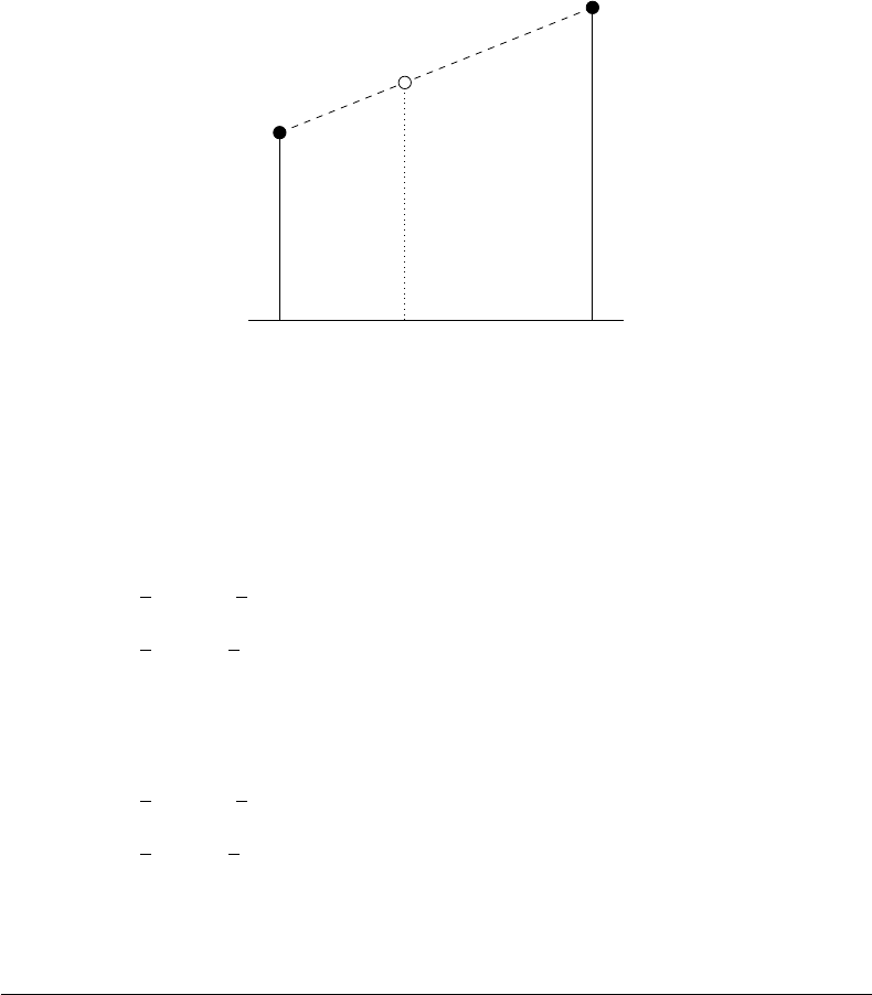
Image Geometry 127
x
1
x
2
f(x
1
)
f(x
2
)
F
λ
1 −λ
FIGURE 6.5: Calculating linearly interpolated values
As an example of how to use this, suppose we have the values f(x
1
) = 2, f(x
2
) = 3,
f(x
3
) = 1.5 and f (x
4
) = 2.5. Consider the point x
4
. This is between x
2
and x
3
, and the
corresponding value for λ is 2/7. Thus
f(x
4
) =
2
7
f(x
3
) +
5
7
f(x
2
)
=
2
7
(1.5) +
5
7
(3)
≈ 2.5714.
For x
7
, we are between x
3
and x
4
with λ = 4/7. So:
f(x
7
) =
4
7
f(x
4
) +
3
7
f(x
3
)
=
4
7
(2.5) +
3
7
(1.5)
≈ 2.0714.
6.2 Image Interpolation
The methods of the previous section can be applied to images. Figure 6.6 shows how a
4 × 4 image would be interpolated to produce an 8 × 8 image. Here the large open circles
are the original points, and the smaller closed circles are the new points.
To obtain function values for the interpolated points, consider the diagram shown in
Figure 6.7.
We can give a value to f(x
, y
) by either of the methods above: by setting it equal to
the function values of the closest image point, or by using linear interpolation. We can
apply linear interpolation first along the top row to obtain a value for f(x, y
), and th en
along the bottom row to obtain a value for f (x + 1, y
). Finally, we can interpolate along
the y
column between these new values to obtain f(x
, y
). Using th e formula given by

128 A Computational Introduction to Digital Image Processing, Second Edition
FIGURE 6.6: Interpolation on an image
(x, y)
(x, y
)
(x, y + 1)
(x
, y) (x
, y + 1)
(x + 1, y)
(x + 1, y
)
(x + 1, y + 1)
(x
, y
)
λ
1 −λ
µ
1 −µ
FIGURE 6.7: Interpolation between four image points

Image Geometry 129
Equation 6.1, then
f(x, y
) = µf (x, y + 1) + (1 − µ)f (x, y)
and
f(x + 1, y
) = µf (x + 1, y + 1) + (1 − µ)f( x + 1, y).
Along the y
column we have
f(x
, y
) = λf (x + 1, y
) + (1 − λ)f(x, y
)
and substituting in the values just obtained produces
f(x
, y
) = λ(µf (x + 1, y + 1) + (1 − µ)f(x + 1, y)) + (1 −λ)(µf (x, y + 1)
+ (1 − µ)f(x, y))
= λµf(x + 1, y + 1) + λ(1 − µ)f(x + 1, y) + (1 −λ)µf (x, y + 1)
+ (1 − λ)(1 − µ)f (x, y)
This last equation is the formula for bilinear interpolation.
Now image scaling can be performed easily. Given our image, and either a scaling factor
(or separate scaling factors for x and y directions), or a size to be scaled to, we first create
an array of the required size. In our example above, we had a 4 ×4 image, given as an array
(x, y), and a scale factor of two, resulting in an array (x
, y
) of size 8 ×8. Going right back
to Figures 6.1 and 6.2, the relationship between (x, y) and (x
, y
) is
(x
, y
) =
1
3
(7x −4),
1
3
(7y − 4)
,
(x, y) =
1
7
(3x
+ 4),
1
7
(3y
+ 4)
.
Given our (x
, y
) array, we can step through it point by point, and from the corresponding
surrounding points from the (x, y) array calculate an interpolated value using either nearest
neighbor or bilinear interpolation.
There’s nothing in the above theory that requires the scaling factor to be greater than
one. We can choose a scaling factor less than one, in which case the resulting image array
will be smaller than the original. We can consider Figure 6.6 in this light: the small closed
circles are the original image points, and the large open circles are the smalle r array on
which we are to find interpolated values.
MATLAB has the function
imresize which does all this for us. It can be called with
imresize(A,k,’method’)
where A is an image of any type, k is a scaling factor, and ’method’ is either ’nearest’ or
’bilinear’ (or another method to be described later). Another way of using imresize is
imresize(A,[m,n],’method’)
where [m,n] provide the size of the scaled output. There is a further, optional parameter
allowing you to choose either the size or type of low pass filter to be applied to the image
before reducing its size—see the help file for details.
Let’s try a few examples. We shall start by taking the head of the cameraman, and
enlarging it by a factor of f our:
..................Content has been hidden....................
You can't read the all page of ebook, please click here login for view all page.