

238 A Computational Introduction to Digital Image Processing, Second Edition
9.7 Derivatives and Edges
Fundamental Definitions
Consider the image in Figure 9.15, and suppose we plot the gray values as we traverse
the image from left to right. Two types of edges are illustrated here: a ramp edge, where the
FIGURE 9.15: Edges and their profiles
gray values change slowly, and a step edge, or an ideal edge, where the gray values change
suddenly.
Suppose the function that provides the profile in Figure 9.15 is f (x); then its derivative
f
(x) can be plotted; this is shown in Figure 9.16. The derivative, as expected, returns zero
0
FIGURE 9.16: The derivative of the edge profile
for all constant sections of the profile, and is non-zero (in this example) only in those parts
of the image in which differences occur.
Many edge finding operators are based on differentiation; to apply the continuous deriva-
tive to a discrete image, first recall the definition of the derivative:
df
dx
= lim
h→0
f(x + h) − f(x)
h
.

Image Segmentation 239
Since in an image, the smallest possible value of h is 1, being the difference between the
index values of two adjacent pixels, a discrete version of the derivative expression is
f(x + 1) − f(x).
Other expressions for the derivative are
lim
h→0
f(x) − f(x − h)
h
, lim
h→0
f(x + h) − f(x − h)
2h
with discrete counterparts
f(x) − f(x − 1), (f(x + 1) − f(x − 1))/2.
For an image, with two dimensions, we use partial derivatives; an important expression is
the gradient, which is the vector defined by
∂f
∂x
∂f
∂y
which for a function f(x, y) points in the direction of its greatest increase. The direction of
that increase is given by
tan
−1
∂f /∂y
∂f /∂x
and its magnitude by
∂f
∂x
2
+
∂f
∂y
2
.
Most edge detection methods are concerned with finding the magnitude of the gradient,
and then applying a threshold to the result.
Some Edge Detection Filters
Using the expression f(x + 1) − f (x − 1) for the derivative, leaving the scaling factor
out, produces horizontal and vertical filters:
−1 0 1
and
−1
0
1
These filters will find vertical and horizontal edges in an image and produce a reasonably
bright result. However, the edges in the result can be a bit “jerky”; this can be overcome
by smoothing the result in the opposite direction; by using the filters
1
1
1
and
1 1 1
Both filters can be applied at once, using the combined filter:
P
x
=
−1 0 1
−1 0 1
−1 0 1
240 A Computational Introduction to Digital Image Processing, Second Edition
This filter, and its companion for finding horizontal edges:
P
y
=
−1 −1 −1
0 0 0
1 1 1
are the Prewitt filters for edge detection.
If p
x
and p
y
are the gray values produced by applying P
x
and P
y
to an image, then the
magnitude of the gradient is obtained with
p
2
x
+ p
2
y
.
In practice, however, it is more convenient to use either of
max{|p
x
|, |p
y
|}
or
|p
x
| + |p
y
|.
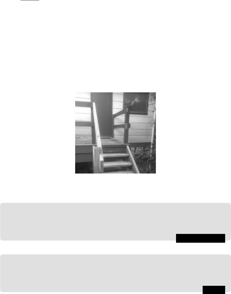
This (and other) edge detection methods will be tested on the image stairs.png,
which we suppose has been read into our system as the array
s. It is shown in Figure 9.17.
Applying each of P
x
and P
y
individually provides the results shown in Figure 9.18 The
FIGURE 9.17: A set of steps: A test image for edge detection
images in Figure 9.18 can be produced with the following MATLAB commands:
MATLAB/Octave
>> px = [-1 0 1;-1 0 1;-1 0 1]; py = px’
>> sx = imfilter(s,px);
>> sy = imfilter(s,py);
>> imshow(sx),figure,imshow(sy)
or these Python commands:
Python
In : sx = fl.hprewitt(s)
In : sy = fl.vprewitt(s)
In : io.imshow(sx)
In : f = plt.figure(); f.show(io.imshow(sy))

Image Segmentation 241
(a) sx (b) sy
FIGURE 9.18: The result after filtering with the Prewitt filters
(There are in fact slight differences in the outputs owing to the way in which each system
manages negative values in the result of a filter.) Note that the filter P
x
highlights vertical
edges, and P
y
horizontal edges. We can create a figure containing all the edges with:
MATLAB/Octave
>> edge
_
p = uint8(sqrt(double(sx).^2+double(sy).^2));
>> figure,imshow(edge
_
p))
or
Python
In : edge
_
p = sqrt(sx
**
2+sy
**
2)
and the result is shown in Figure 9.19(a). This is a grayscale image; a binary image
containing edges only can be produced by thresholding. Figure 9.19(b) shows the result
after thresholding with a value found by Otsu’s method; this optimum threshold value is
0.3333.
(a) (b)
FIGURE 9.19: All the edges of the image

242 A Computational Introduction to Digital Image Processing, Second Edition
We can obtain edges by the Prewitt filters directly in MATLAB or Octave by using the
command
MATLAB/Octave
>> edge
_
p = edge(s,’prewitt’);
and the
edge
function takes care of all the filtering, and of choosing a suitable threshold
level; see its help text for more information. The result is shown in Figure 9.20. Note that
FIGURE 9.20: The prewitt option of edge
Figures 9.19(b) and 9.20 seem different from each other. This is because the
edge
function
does some extra processing over and above taking the square root of the sum of the squares
of the filters.
Python does not have a function that automatically computes threshold values and
cleans up the output. However, in Chapter 10, we will see how to clean up binary images.
Slightly different edge finding filters are the Roberts cross-gradient filters:
1 0 0
0 −1 0
0 0 0
and
0 1 0
−1 0 0
0 0 0
and the Sobel filters:
−1 0 1
−2 0 2
−1 0 1
and
−1 −2 1
0 0 0
1 2 1
.
The Sobel filters are similar to the Prewitt filters in that they apply a smoothing filter in
the opposite direction to the central difference filter. In the Sobel filters, the smoothing
takes the form
1 2 1
which gives slightly more prominence to the central pixel. Figure 9.21 shows the respective
results of the MATLAB/Octave commands
MATLAB/Octave
>> edge
_
r = edge(s,’roberts’);
>> figure,imshow(edge
_
r)
..................Content has been hidden....................
You can't read the all page of ebook, please click here login for view all page.