

Chapter 13
Color Processing
For human beings, color provides one of the most imp ortant descriptors of the world around
us. The human visual system is particularly attuned to two things: edges and color. We
have mentioned that the human visual system is not particularly good at recognizing subtle
changes in gray values. In this section we shall investigate color briefly, and then some
methods of processing color images
13.1 What Is Color?
Color study consists of
1. The physical properties of light which give rise to color
2. The nature of the human eye and the ways in which it detects color
3. The nature of the human vision center in the brain, and the ways in which messages
from the eye are perceived as color
Physical Aspects of Color
As we have seen in Chapter 1, visible light is part of the electromagnetic spectrum. The
values for the wavelengths of blue, green, and red were set in 1931 by the CIE (Commission
Internationale d’Eclairage), an organization responsible for color standards.
Perceptual Aspects of Color
The human visual system tends to perceive color as being made up of varying amounts
of red, green, and blue. That is, human vision is particularly sensitive to these colors; this
is a function of the cone cells in the retina of the eye. These values are called the primary
colors. If we add together any two primary colors, we obtain the secondary colors:
magenta (purple) = red + blue
cyan = green + blue
yellow = red + green
The amounts of red, green, and blue that make up a given color can be determined by a
color matching experiment. In such an experiment, people are asked to match a given color
(a color source) with different amounts of the additive primaries red, green, and blue. Such
an experiment was performed in 1931 by the CIE, and the results are shown in Figure 13.1.
Note that for some wavelengths, various red, green, or blue values are negative. This is a
371

372 A Computational Introduction to Digital Image Processing, Second Edition
FIGURE 13.1: RGB color matching functions (CIE, 1931)
physical impossibility, but it can be interpreted by adding the primary beam to the color
source, to maintain a color match.
To remove negative values from color information, the CIE introduced the XYZ color
model. The values of X, Y , and Z can be obtained from the corresponding R, G, and B
values by a linear transformation:
X
Y
Z
=
0.431 0.342 0.178
0.222 0.707 0.071
0.020 0.130 0.939
R
G
B
The inverse transf ormation is easily obtained by inverting the matrix:
R
G
B
=
3.063 −1.393 −0.476
−0.969 1.876 0.042
0.068 −0.229 1.069
X
Y
Z
The XYZ color matching functions corresponding to the R, G, B curves of Figure 13.1
are shown in Figure 13.2. The matrices given are not fixed; other matrices can be defined
according to the definition of the color white. Different definitions of white will lead to
different transformation matrices.
The CIE required that the Y component corresponded with luminance, or perceived
brightness of the color. That is why the row corresponding to Y in the first matrix (that
is, the second row) sums to 1, and also why the Y curve in Figure 13.2 is symmetric about
the middle of the visible spectrum.
In general, the values of X, Y , and Z needed to form any particular color are called the
tristimulus values. Values corresponding to particular colors can be obtained from published
tables. In order to discuss color independent of brightness, the tristimulus values can be

Color Processing 373
FIGURE 13.2: XYZ color matching functions (CIE, 1931)
normalized by dividing by X + Y + Z:
x =
X
X + Y + Z
y =
Y
X + Y + Z
z =
Z
X + Y + Z
and so x+y +z = 1. Thus, a color can be specified by x and y alone, called the chromaticity
coordinates. Given x, y, and Y , we can obtain the tristimulus values X and Z by working
through the above equations backward:
X =
x
y
Y
Z =
1 −x − y
y
Y.
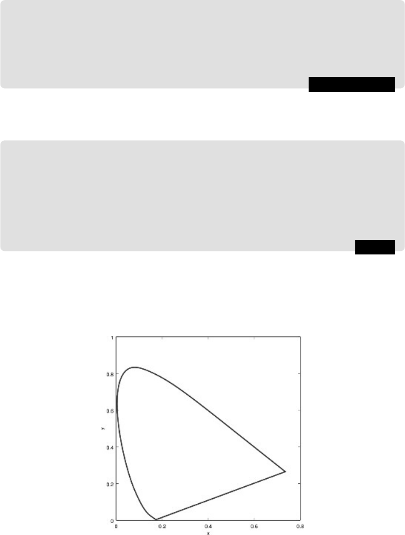
We can plot a chromaticity diagram, using the
ciexyz31.csv
1
file of XYZ values. In
MATLAB/Octave:
1
This file can be obtained from the Color & Vision Research Laboratories web page
http://www.cvrl.org.
374 A Computational Introduction to Digital Image Processing, Second Edition
MATLAB/Octave
>> nxyz = dlmread(’ciexyz31.csv’);
>> xyz = wxyz(:,2:4)’;
>> xy = xyz’./(
sum
(xyz)’
*
[1 1 1]);
>> x = xy(:,1)’;
>> y = xy(:,2)’;
>> figure,plot([x x(1)],[y y(1)]),xlabel(’x’),ylabel(’y’),axis square
In Python:
Python
In : import matplotlib.pyplot as plt
In : nxyz = np.loadtxt(’ciexyz31
_
1.csv’,delimiter=’,’)
In : xyz = nxyz[:,1:]
In : sums = xyz.sum(axis=1)
In : newxyz = xyz/sums[:,np.newaxis]
In : x = newxyz[0,:]; x1 = np.hstack((x,x[0]))
In : y = newxyz[1,:]; y1 = np.hstack((y,y[0]))
In : plt.plot(x1,y1)
Here the matrix
xyz
consists of the second, third, and fourth columns of the d ata, and
plot
is a function that draws a polygon with vertices taken from the x and y vectors. The extra
x(1) and y(1) ensures that the polygon joins up. The result is shown in Figure 13.3. The
FIGURE 13.3: A chromaticity diagram
values of x and y that lie within the horseshoe shape in Figure 13.3 represent values that
correspond to physically realizable colors. A good account of the XYZ model and associated
color theory can be f ound in Foley et al. [11].
Color Processing 375
13.2 Color Models
A color model is a method for specifying colors in some standard way. It generally
consists of a three-dimensional coordinate system and a subspace of that system in which
each color is represented by a single point. We shall investigate three systems.
RGB
In this model, each color is represented as three values R, G, and B, indicating the
amounts of red, green, and blue which make up the color. This model is used for displays
on computer screens; a monitor has three independent electron “guns” for the red, green,
and blue component of each color. We have met this model in Chapter 2.
Note also from Figure 13.1 that some colors require negative values of R, G or B. These
colors are not realizable on a computer monitor or TV set, on which only positive values
are possible. The colors corresponding to positive values form the RGB gamut; in general
a color “gamut” consists of all the colors realizable with a particular color model. We can
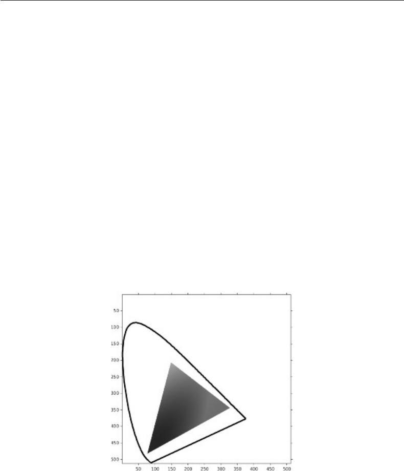
plot the RGB gamut on a chromaticity diagram, using the
xy coordinates obtained above.
To define the gamut, we shall create a 100 × 100 × 3 array, and to each point (i, j) in the
array, associate an XYZ triple defined by (i/100, j/100, 1 − i/100 − j/100). We can then
compute the corresponding RGB triple, and if any of the RGB values are negative, make
the output value white. Programs to display the gamut, which is shown in Figure 13.4, are
given at the end of the chapter
FIGURE 13.4: SEE COLOR INSERT The RGB gamut
HSV
HSV stands for hue, saturation, and value. These terms have the following meanings:
Hue: The “true color” attribute (red, green, blue, orange, yellow, and so on).
Saturation: The amount by which the color has been diluted with white. The more white
in the color, the lower the saturation. So a deep red has high saturation, and a light
red (a pinkish color) has low saturation.
..................Content has been hidden....................
You can't read the all page of ebook, please click here login for view all page.