2
Errors & Uncertainties in Computations
To err is human, to forgive divine.
— Alexander Pope
Whether you are careful or not, errors and uncertainties are a part of computation. Some errors are the ones that humans inevitably make, but some are introduced by the computer. Computer errors arise because of the limited precision with which computers store numbers or because algorithms or models can fail. Although it stifles creativity to keep thinking “error” when approaching a computation, it certainly is a waste of time, and may lead to harm, to work with results that are meaningless (“garbage”) because of errors. In this chapter we examine some of the errors and uncertainties that may occur in computations. Even though we do not dwell on it, the lessons of this chapter apply to all other chapters as well.
2.1 Types of Errors (Theory)
Let us say that you have a program of high complexity. To gauge why errors should be of concern, imagine a program with the logical flow
where each unit U might be a statement or a step. If each unit has probability p of being correct, then the joint probability P of the whole program being correct is P = pn. Let us say we have a medium-sized program with n = 1000 steps and that the probability of each step being correct is almost one, p ![]() 0.9993. This means that you end up with P
0.9993. This means that you end up with P ![]()
![]() , that is, a final answer that is as likely wrong as right (not a good way to build a bridge). The problem is that, as a scientist, you want a result that is correct—or at least in which the uncertainty is small and of known size.
, that is, a final answer that is as likely wrong as right (not a good way to build a bridge). The problem is that, as a scientist, you want a result that is correct—or at least in which the uncertainty is small and of known size.
Four general types of errors exist to plague your computations:
Blunders or bad theory: typographical errors entered with your program or data, running the wrong program or having a fault in your reasoning (theory), using the wrong data file, and so on. (If your blunder count starts increasing, it may be time to go home or take a break.)
Random errors: imprecision caused by events such as fluctuations in electronics, cosmic rays, or someone pulling a plug. These may be rare, but you have no control over them and their likelihood increases with running time; while you may have confidence in a 20-s calculation, a week-long calculation may have to be run several times to check reproducibility.
Approximation errors: imprecision arising from simplifying the mathematics so that a problem can be solved on the computer. They include the replacement of infinite series by finite sums, infinitesimal intervals by finite ones, and variable functions by constants. For example,
where ε(x, N) is the approximation error and where in this case ε is the series from N +1 to ∞. Because approximation error arises from the algorithm we use to approximate the mathematics, it is also called algorithmic error. For every reasonable approximation, the approximation error should decrease as N increases and vanish in the N —> ∞ limit. Specifically for (2.2), because the scale for N is set by the value of x, a small approximation error requires N
x. So if x and N are close in value, the approximation error will be large.
Round-off errors: imprecision arising from the finite number of digits used to store floating-point numbers. These “errors” are analogous to the uncertainty in the measurement of a physical quantity encountered in an elementary physics laboratory. The overall round-off error accumulates as the computer handles more numbers, that is, as the number of steps in a computation increases, and may cause some algorithms to become unstable with a rapid increase in error. In some cases, round-off error may become the major component in your answer, leading to what computer experts call garbage. For example, if your computer kept four decimal places, then it will store
as 0.3333 and
as 0.6667, where the computer has “rounded off” the last digit in


So even though the result is small, it is not 0, and if we repeat this type of calculation millions of times, the final answer might not even be small (garbage begets garbage).
When considering the precision of calculations, it is good to recall our discussion in Chapter 1, “Computational Science Basics,” of significant figures and of scientific notation given in your early physics or engineering classes. For computational purposes, let us consider how the computer may store the floating-point number
Because the exponent is stored separately and is a small number, we can assume that it will be stored in full precision. In contrast, some of the digits of the mantissa may be truncated. In double precision the mantissa of a will be stored in two words, the most significant part representing the decimal 1.12233, and the least significant part 44556677. The digits beyond 7 are lost. As we see below, when we perform calculations with words of fixed length, it is inevitable that errors will be introduced (at least) into the least significant parts of the words.
2.1.1 Model for Disaster: Subtractive Cancellation
A calculation employing numbers that are stored only approximately on the computer can be expected to yield only an approximate answer. To demonstrate the effect of this type of uncertainty, we model the computer representation xc of the exact number x as
![]()
Here εx is the relative error in xc, which we expect to be of a similar magnitude to the machine precision εm. If we apply this notation to the simple subtraction a = b - c, we obtain
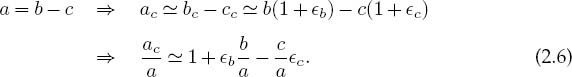
We see from (2.6) that the resulting error in a is essentially a weighted average of the errors in b and c, with no assurance that the last two terms will cancel. Of special importance here is to observe that the error in the answer ac increases when we subtract two nearly equal numbers (b ![]() c) because then we are subtracting off the most significant parts of both numbers and leaving the error-prone least-significant parts:
c) because then we are subtracting off the most significant parts of both numbers and leaving the error-prone least-significant parts:
![]()
This shows that even if the relative errors in b and c may cancel somewhat, they are multiplied by the large number b/a, which can significantly magnify the error. Because we cannot assume any sign for the errors, we must assume the worst [the “max” in (2.7)].
If you subtract two large numbers and end up with a small one, there will be less significance, and possibly a lot less significance, in the small one.
We have already seen an example of subtractive cancellation in the power series summation for sin x ![]() x – x3/3! + ••• for large x. A similar effect occurs for e-x
x – x3/3! + ••• for large x. A similar effect occurs for e-x ![]() 1 - x + x2/2! – x3/3! + ••• for large x, where the first few terms are large but of alternating sign, leading to an almost total cancellation in order to yield the final small result. (Subtractive cancellation can be eliminated by using the identity e-x = 1/ex, although round-off error will still remain.)
1 - x + x2/2! – x3/3! + ••• for large x, where the first few terms are large but of alternating sign, leading to an almost total cancellation in order to yield the final small result. (Subtractive cancellation can be eliminated by using the identity e-x = 1/ex, although round-off error will still remain.)
2.1.2 Subtractive Cancellation Exercises
1. Remember back in high school when you learned that the quadratic equation
has an analytic solution that can be written as either

Inspection of (2.9) indicates that subtractive cancellation (and consequently an increase in error) arises when b2 ![]() 4ac because then the square root and its preceding term nearly cancel for one of the roots.
4ac because then the square root and its preceding term nearly cancel for one of the roots.
a. Write a program that calculates all four solutions for arbitrary values of a, b, and c.
b. Investigate how errors in your computed answers become large as the subtractive cancellation increases and relate this to the known machine precision. (Hint: A good test case employs a = 1, b = 1, c = 10-n, n = 1, 2, 3,….)
c. Extend your program so that it indicates the most precise solutions.
2. As we have seen, subtractive cancellation occurs when summing a series with alternating signs. As another example, consider the finite sum

If you sum the even and odd values of n separately, you get two sums:

All terms are positive in this form with just a single subtraction at the end of the calculation. Yet even this one subtraction and its resulting cancellation can be avoided by combining the series analytically to obtain
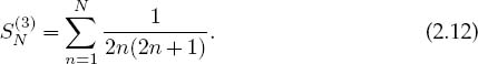
Even though all three summations S(1), S(2), and S(3) are mathematically equal, they may give different numerical results.
a. Write a single-precision program that calculates S(1), S(2), and S(3).
b. Assume S(3) to be the exact answer. Make a log-log plot of the relative error versus the number of terms, that is, of log10 |(SN(1) –SN(3))/SN(3)| versus log10(N). Start with N = 1 and work up to N = 1,000,000. (Recollect that log10 x = ln x/ ln 10.) The negative of the ordinate in this plot gives an approximate value for the number of significant figures.
c. See whether straight-line behavior for the error occurs in some region of your plot. This indicates that the error is proportional to a power of N.
3. In spite of the power of your trusty computer, calculating the sum of even a simple series may require some thought and care. Consider the two series
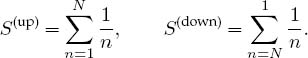
Both series are finite as long as N is finite, and when summed analytically both give the same answer. Nonetheless, because of round-off error, the numerical value of S(up) will not be precisely that of S(down).
a. Write a program to calculate S(up) and S(down) as functions of N.
b. Make a log-log plot of (S(up) -S(down))/(|S(up)|+|S(down)|) versus N.
c. Observe the linear regime on your graph and explain why the downward sum is generally more precise.
![]()
2.1.3 Round-off Error in a Single Step
Let’s start by seeing how error arises from a single division of the computer representations of two numbers:

Here we ignore the very small ε2 terms and add errors in absolute value since we cannot assume that we are fortunate enough to have unknown errors cancel each other. Because we add the errors in absolute value, this same rule holds for multiplication. Equation (2.13) is just the basic rule of error propagation from elementary laboratory work: You add the uncertainties in each quantity involved in an analysis to arrive at the overall uncertainty.
We can even generalize this model to estimate the error in the evaluation of a general function f (x), that is, the difference in the value of the function evaluated at x and at xc:
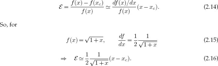
If we evaluate this expression for x = π/4 and assume an error in the fourth place of x, we obtain a similar relative error of 1.5 × 10⁻⁴ in ![]() .
.
2.1.4 Round-off Error Accumulation After Many Steps
There is a useful model for approximating how round-off error accumulates in a calculation involving a large number of steps. We view the error in each step as a literal “step” in a random walk, that is, a walk for which each step is in a random direction. As we derive and simulate in Chapter 5, “Monte Carlo Simulations,” the total distance covered in N steps of length r, is, on the average,
![]()
By analogy, the total relative error εro arising after N calculational steps each with machine precision error εm is, on the average,
![]()
If the round-off errors in a particular algorithm do not accumulate in a random manner, then a detailed analysis is needed to predict the dependence of the error on the number of steps N. In some cases there may be no cancellation, and the error may increase as Nεm. Even worse, in some recursive algorithms, where the error generation is coherent, such as the upward recursion for Bessel functions, the error increases as N!.
Our discussion of errors has an important implication for a student to keep in mind before being impressed by a calculation requiring hours of supercomputer time. A fast computer may complete 1010 floating-point operations per second. This means that a program running for 3 h performs approximately 1014 operations. Therefore, if round-off error accumulates randomly, after 3 h we expect a relative error of 107εm. For the error to be smaller than the answer, we need εm < 10-7, which requires double precision and a good algorithm. If we want a higher-precision answer, then we will need a very good algorithm.
2.2 Errors in Spherical Bessel Functions (Problem)
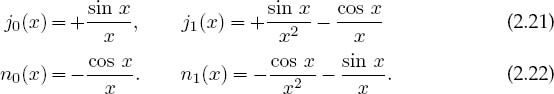
Accumulating round-off errors often limits the ability of a program to calculate accurately. Your problem is to compute the spherical Bessel and Neumann functions jl(x) and nl (x). These function are, respectively, the regular/irregular (nonsingular/singular at the origin) solutions of the differential equation
The spherical Bessel functions are related to the Bessel function of the first kind by ![]() . They occur in many physical problems, such as the expansion of a plane wave into spherical partial waves,
. They occur in many physical problems, such as the expansion of a plane wave into spherical partial waves,

Figure 2.1 shows what the first few jl look like, and Table 2.1 gives some explicit values. For the first two l values, explicit forms are
2.2.1 Numerical Recursion Relations (Method)
The classic way to calculate jl(x) would be by summing its power series for small values of x/l and summing its asymptotic expansion for large x values. The approach we adopt is based on the recursion relations
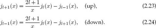
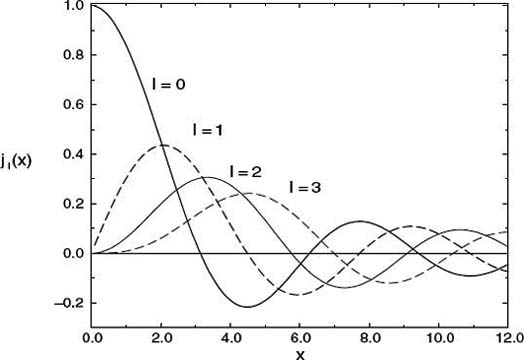
Figure 2.1 The first four spherical Bessel functions jl (x) as functions of x. Notice that for small x, the values for increasing l become progressively smaller.
TABLE 2.1
Approximate Values for Spherical Bessel Functions of Orders 3, 5, and 8 (from Maple)
x |
j3(x) |
j5(x) |
j8(x) |
0.1 |
+9.518519719 10-6 |
+9.616310231 10-10 |
+2.901200102 10-16 |
1 |
+9.006581118 10-3 |
+9.256115862 10-05 |
+2.826498802 10-08 |
10 |
-3.949584498 10-2 |
-5.553451162 10-01 |
+1.255780236 10+00 |
Equations (2.23) and (2.24) are the same relation, one written for upward recurrence from small to large l values, and the other for downward recurrence to small l values. With just a few additions and multiplications, recurrence relations permit rapid, simple computation of the entire set of jl values for fixed x and all l.
To recur upward in l for fixed x, we start with the known forms for jo and j1 (2.21) and use (2.23). As you will prove for yourself, this upward recurrence usually seems to work at first but then fails. The reason for the failure can be seen from the plots of jl(x) and nl (x) versus x (Figure 2.1). If we start at x ![]() 2 and l = 0, we will see that as we recur jl up to larger l values with (2.23), we are essentially taking the difference of two “large” functions to produce a “small” value for jl. This process suffers from subtractive cancellation and always reduces the precision. As we continue recurring, we take the difference of two small functions with large errors and produce a smaller function with yet a larger error. After a while, we are left with only round-off error (garbage).
2 and l = 0, we will see that as we recur jl up to larger l values with (2.23), we are essentially taking the difference of two “large” functions to produce a “small” value for jl. This process suffers from subtractive cancellation and always reduces the precision. As we continue recurring, we take the difference of two small functions with large errors and produce a smaller function with yet a larger error. After a while, we are left with only round-off error (garbage).
To be more specific, let us call jl(c) the numerical value we compute as an approximation for jl(x). Even if we start with pure jl, after a short while the computer’s lack of precision effectively mixes in a bit of nl(x):
This is inevitable because both jl and nl satisfy the same differential equation and, on that account, the same recurrence relation. The admixture of nl becomes a problem when the numerical value of nl(x)is much larger than that of jl(x) because even a minuscule amount of a very large number may be large. In contrast, if we use the upward recurrence relation (2.23) to produce the spherical Neumann function nl, there will be no problem because we are combining small functions to produce larger ones (Figure 2.1), a process that does not contain subtractive cancellation.
The simple solution to this problem (Miller’s device) is to use (2.24) for downward recursion of the jl values starting at a large value l = L. This avoids subtractive cancellation by taking small values of jl+1(x) and jl(x) and producing a larger jl-1(x) by addition. While the error may still behave like a Neumann function, the actual magnitude of the error will decrease quickly as we move downward to smaller l values. In fact, if we start iterating downward with arbitrary values for jL+1(c) and jL(c), after a short while we will arrive at the correct l dependence for this value of x. Although the numerical value of j0(c) so obtained will not be correct because it depends upon the arbitrary values assumed forjL+1(c) and jL(c), the relative values will be accurate. The absolute values are fixed from the know value (2.21), j0(x) = sin x/x. Because the recurrence relation is a linear relation between the jl values, we need only normalize all the computed values via
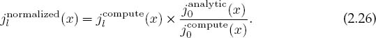
Accordingly, after you have finished the downward recurrence, you obtain the final answer by normalizing all jl(c) values based on the known value for j0.
2.2.2 Implementation and Assessment: Recursion Relations
A program implementing recurrence relations is most easily written using subscripts. If you need to polish up on your skills with subscripts, you may want to study our program Bessel.java in Listing 2.1 before writing your own.
1. Write a program that uses both upward and downward recursion to calculate jl(x) for the first 25 l values for x = 0.1,1,10.
2. Tune your program so that at least one method gives “good” values (meaning a relative error ![]() 10-10). See Table 2.1 for some sample values.
10-10). See Table 2.1 for some sample values.
3. Show the convergence and stability of your results.
4. Compare the upward and downward recursion methods, printing out l, jl(up), jl(down), and the relative difference |jl(up) - jl(down)|/|jl(up)| + |jl(down)|.
5. The errors in computation depend on x, and for certain values of x, both up and down recursions give similar answers. Explain the reason for this.
![]()

Listing 2.1 Bessel.java determines spherical Bessel functions by downward recursion (you should modify this to also work by upward recursion).
2.3 Experimental Error Investigation (Problem)
Numerical algorithms play a vital role in computational physics. Your problem is to take a general algorithm and decide
1. Does it converge?
2. How precise are the converged results?
3. How expensive (time-consuming) is it?
On first thought you may think, “What a dumb problem!All algorithms converge if enough terms are used, and if you want more precision, then use more terms.” Well, some algorithms may be asymptotic expansions that just approximate a function in certain regions of parameter space and converge only up to a point. Yet even if a uniformly convergent power series is used as the algorithm, including more terms will decrease the algorithmic error but increase the round-off errors. And because round-off errors eventually diverge to infinity, the best we can hope for is a “best” approximation. Good algorithms are good not only because they are fast but also because being fast means that round-off error does not have much time to grow.
Let us assume that an algorithm takes N steps to find a good answer. As a rule of thumb, the approximation (algorithmic) error decreases rapidly, often as the inverse power of the number of terms used:
Here α and β are empirical constants that change for different algorithms and may be only approximately constant, and even then only as N → ∞. The fact that the error must fall off for large N is just a statement that the algorithm converges.
In contrast to this algorithmic error, round-off error tends to grow slowly and somewhat randomly with N. If the round-off errors in each step of the algorithm are not correlated, then we know from previous discussion that we can model the accumulation of error as a random walk with step size equal to the machine precision εm:
![]()
This is the slow growth with N that we expect from round-off error. The total error in a computation is the sum of the two types of errors:

For small N we expect the first term to be the larger of the two but ultimately to be overcome by the slowly growing round-off error.
As an example, in Figure 2.2 we present a log-log plot of the relative error in numerical integration using the Simpson integration rule (Chapter 6, “Integration”). We use the log10 of the relative error because its negative tells us the number of decimal places of precision obtained.1 As a case in point, let us assume A is the exact answer and A(N) the computed answer. If

We see in Figure 2.2 that the error does show a rapid decrease for small N, consistent with an inverse power law (2.27). In this region the algorithm is converging. As N is increased, the error starts to look somewhat erratic, with a slow increase on the average. In accordance with (2.29), in this region round-off error has grown larger than the approximation error and will continue to grow for increasing N. Clearly then, the smallest total error will be obtained if we can stop the calculation at the minimum near 10-14, that is, when εapprox ![]() εro.
εro.

Figure 2.2 A log-log plot of relative error versus the number of points used for a numerical integration. The ordinate value of ![]() 10-14 at the minimum indicates that ~14 decimal places of precision are obtained before round-off error begins to build up. Notice that while the round-off error does fluctuate, on the average it increases slowly.
10-14 at the minimum indicates that ~14 decimal places of precision are obtained before round-off error begins to build up. Notice that while the round-off error does fluctuate, on the average it increases slowly.
In realistic calculations you would not know the exact answer; after all, if you did, then why would you bother with the computation? However, you may know the exact answer for a similar calculation, and you can use that similar calculation to perfect your numerical technique. Alternatively, now that you understand how the total error in a computation behaves, you should be able to look at a table or, better yet, a graph (Figure 2.2) of your answer and deduce the manner in which your algorithm is converging. Specifically, at some point you should see that the mantissa of the answer changes only in the less significant digits, with that place moving further to the right of the decimal point as the calculation executes more steps. Eventually, however, as the number of steps becomes even larger, round-off error leads to a fluctuation in the less significant digits, with a gradual increase on the average. It is best to quit the calculation before this occurs.
Based upon this understanding, an approach to obtaining the best approximation is to deduce when your answer behaves like (2.29). To do that, we call A the exact answer and A(N) the computed answer after N steps. We assume that for large enough values of N, the approximation converges as
that is, that the round-off error term in (2.29) is still small. We then run our computer program with 2N steps, which should give a better answer, and use that answer to eliminate the unknown A:
![]()
To see if these assumptions are correct and determine what level of precision is possible for the best choice of N, plot log10 |[A(N) – A(2N)]/A(2N)| versus log10 N, similar to what we have done in Figure 2.2. If you obtain a rapid straight-line drop off, then you know you are in the region of convergence and can deduce a value for β from the slope. As N gets larger, you should see the graph change from a straight-line decrease to a slow increase as round-off error begins to dominate. A good place to quit is before this. In any case, now you understand the error in your computation and therefore have a chance to control it.
As an example of how different kinds of errors enter into a computation, we assume we know the analytic form for the approximation and round-off errors:
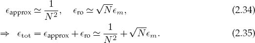
The total error is then a minimum when

For a single-precision calculation (εm ![]() 10 -7), the minimum total error occurs when
10 -7), the minimum total error occurs when
![]()
In this case most of the error is due to round-off and is not approximation error. Observe, too, that even though this is the minimum total error, the best we can do is about 40 times machine precision (in double precision the results are better).
Seeing that the total error is mainly round-off error ∝ ![]() , an obvious way to decrease the error is to use a smaller number of steps N. Let us assume we do this by finding another algorithm that converges more rapidly with N, for example, one with approximation error behaving like
, an obvious way to decrease the error is to use a smaller number of steps N. Let us assume we do this by finding another algorithm that converges more rapidly with N, for example, one with approximation error behaving like
![]()
The total error is now
![]()
The number of points for minimum error is found as before:
![]()

Figure 2.3 The error in the summation of the series for e-x versus N. The values of x increase vertically for each curve. Note that a negative initial slope corresponds to decreasing error with N, and that the dip corresponds to a rapid convergence followed by a rapid increase in error. (Courtesy of J. Wiren.)
The error is now smaller by a factor of 4, with only ![]() as many steps needed. Subtle are the ways of the computer. In this case the better algorithm is quicker and, by using fewer steps, it produces less round-off error.
as many steps needed. Subtle are the ways of the computer. In this case the better algorithm is quicker and, by using fewer steps, it produces less round-off error.
Exercise: Repeat the error estimates for a double-precision calculation.
![]()
2.3.1 Error Assessment
We have already discussed the Taylor expansion of sin x:

This series converges in the mathematical sense for all values of x. Accordingly, a reasonable algorithm to compute the sin(x) might be

While in principle it should be faster to see the effects of error accumulation in this algorithm by using single-precision numbers, C and Java tend to use double-precision mathematical libraries, and so it is hard to do a pure single-precision computation. Accordingly, do these exercises in double precision, as you should for all scientific calculations involving floating-point numbers.
1. Write a program that calculates sin(x) as the finite sum (2.43). (If you already did this in Chapter 1, “Computational Science Basics,” then you may reuse that program and its results here.)
2. Calculate your series for x ≤ 1 and compare it to the built-in function Math.sin(x) (you may assume that the built-in function is exact). Stop your summation at an N value for which the next term in the series will be no more than 10-7 of the sum up to that point,

3. Examine the terms in the series for x ![]() 3π and observe the significant subtractive cancellations that occur when large terms add together to give small answers. [Do not use the identity sin(x +2π) = sin x to reduce the value of x in the series.] In particular, print out the near-perfect cancellation around n
3π and observe the significant subtractive cancellations that occur when large terms add together to give small answers. [Do not use the identity sin(x +2π) = sin x to reduce the value of x in the series.] In particular, print out the near-perfect cancellation around n ![]() x/2.
x/2.
4. See if better precision is obtained by using trigonometric identities to keep 0 < x < π.
5. By progressively increasing x from 1 to 10, and then from 10 to 100, use your program to determine experimentally when the series starts to lose accuracy and when it no longer converges.
6. Make a series of graphs of the error versus N for different values of x. (See Chapter 3, “Visualization Tools.”) You should get curves similar to those in Figure 2.3.
![]()
Because this series summation is such a simple, correlated process, the round-off error does not accumulate randomly as it might for a more complicated computation, and we do not obtain the error behavior (2.32). We will see the predicted error behavior when we examine integration rules in Chapter 6, “Integration.”
1 Most computer languages use ln x = loge x. Yet since x = alogax, we have log10 x = lnx/ ln 10.