8
Solving Systems of Equations with Matrices; Data Fitting
Unit I of this chapter applies the trial-and-error techniques developed in Chapter 7, “Differentiation & Searching,” to solve a set of simultaneous nonlinear equations. This leads us into general matrix computing using scientific libraries. In Unit II we look at several ways in which theoretical formulas are fit to data and see that these often require the matrix techniques of Unit I.
8.1 Unit I. Systems of Equations and Matrix Computing
Physical systems are often modeled by systems of simultaneous equations written in matrix form. As the models are made more realistic, the matrices often become large, and computers become an excellent tool for solving such problems. What makes computers so good is that matrix manipulations intrinsically involve the continued repetition of a small number of simple instructions, and algorithms exist to do this quite efficiently. Further speedup may be achieved by tuning the codes to the computer’s architecture, as discussed in Chapter 14, “High-Performance Computing Hardware, Tuning, & Parallel Computing.”
Industrial-strength subroutines for matrix computing are found in well-established scientific libraries. These subroutines are usually an order of magnitude or more faster than the elementary methods found in linear algebra texts,1 are usually designed to minimize round-off error, and are often “robust,” that is, have a high chance of being successful for a broad class of problems. For these reasons we recommend that you do not write your own matrix subroutines but instead get them from a library. An additional value of library routines is that you can often run the same program either on a desktop machine or on a parallel supercomputer, with matrix routines automatically adapting to the local architecture.
The thoughtful reader may be wondering when a matrix is “large” enough to require the use of a library routine. While in the past large may have meant a good fraction of your computer’s random-access memory (RAM), we now advise that a library routine be used whenever the matrix computations aresonumerically intensive that you must wait for results. In fact, even if the sizes of your matrices are small, as may occuringraphical processing, there maybe library routines designed just for that which speed up your computation.
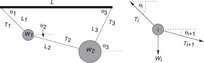
Figure 8.1 Left: Two weights connected by three pieces of string and suspended from a horizontal bar of length L. The angles and the tensions in the strings are unknown. Right: A free body diagram for one weight in equilibrium.
Now that you have heard the sales pitch, you may be asking, “What’s the cost?” In the later part of this chapter we pay the costs of having to find what libraries are available, of having to find the name of the routine in that library, of having to find the names of the subroutines your routine calls, and then of having to figure out how to call all these routines properly. And because some of the libraries are in Fortran, if you are a C programmer you may also be taxed by having to call a Fortran routine from your C program. However, there are now libraries available in most languages.
8.2 Two Masses on a String
Two weights (W1,W2) = (10,20) are hung from three pieces of string with lengths (L1,L2,L3) = (3,4,4)and a horizontal bar of length L = 8(Figure8.1). The problem is to find the angles assumed by the strings and the tensions exerted by the strings.
In spite of the fact that this is a simple problem requiring no more than first-year physics to formulate, the coupled transcendental equations that result are inhumanely painful to solve analytically. However, we will show you how the computer can solve this problem, but even then only by a trial-and-error technique with no guarantee of success. Your problem is to test this solution for a variety of weights and lengths and then to extend it to the three-weight problem (not as easy as it may seem). In either case check the physical reasonableness of your solution; the deduced tensions should be positive and of similar magnitude to the weights of the spheres, and the deduced angles should correspond to a physically realizable geometry, as confirmed with a sketch. Some of the exploration you should do is to see at what point your initial guess gets so bad that the computer is unable to find a physical solution.
8.2.1 Statics (Theory)
We start with the geometric constraints that the horizontal length of the structure is L and that the strings begin and end at the same height (Figure 8.1 left):
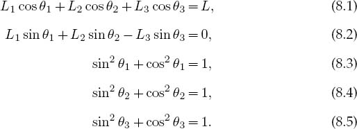
Observe that the last three equations include trigonometric identities as independent equations because we are treating sinθ and cosθ as independent variables; this makes the search procedure easier to implement. The basics physics says that since there are no accelerations, the sum of the forces in the horizontal and vertical directions must equal zero (Figure 8.1 right):
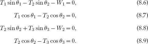
Here Wi is the weight of mass i and Ti is the tension in string i. Note that since we do not have a rigid structure, we cannot assume the equilibrium of torques.
8.2.2 Multidimensional Newton–Raphson Searching
Equations (8.1)–(8.9) are nine simultaneous nonlinear equations. While linear equations can be solved directly, nonlinear equations cannot [Pres 00]. You can use the computer to search for a solution by guessing, but there is no guarantee of finding one. We apply to our set the same Newton–Raphson algorithm as used to solve a single equation by renaming the nine unknown angles and tensions as the subscripted variable yi and placing the variables together as a vector:
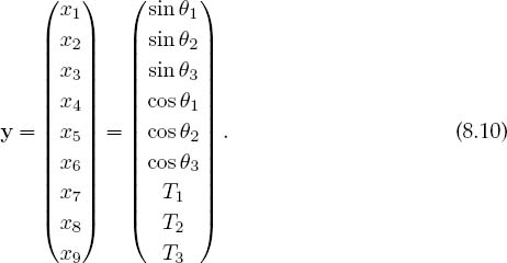
The nine equations to be solved are written in a general form with zeros on the right-hand sides and placed in a vector:
The solution to these equations requires a set of nine xi values that make all nine f i’s vanish simultaneously. Although these equations are not very complicated (the physics after all is elementary), the terms quadratic in x make them nonlinear, and this makes it hard or impossible to find an analytic solution. The search algorithm is to guess a solution, expand the nonlinear equations into linear form, solve the resulting linear equations, and continue to improve the guesses based on how close the previous one was to making f = 0.
Explicitly, let the approximate solution at any one stage be the set {xi} and let us assume that there is an (unknown) set of corrections {∆xi} for which
![]()
We solve for the approximate ∆xi’s by assuming that our previous solution is close enough to the actual one for two terms in the Taylor series to be accurate:

We now have a solvable set of nine linear equations in the nine unknowns ∆xi, which we express as a single matrix equation

Note now that the derivatives and the f’s are all evaluated at known values of the xi’s, so only the vector of the ∆xi values is unknown. We write this equation in matrix notation as

Here we use bold to emphasize the vector nature of the columns of fi and ∆xi values and call the matrix of the derivatives F’ (it is also sometimes called J because it is the Jacobian matrix).
The equation F’∆x = —f is in the standard form for the solution of a linear equation (often written Ax = b), where ∆x is the vector of unknowns and b = — f. Matrix equations are solved using the techniques of linear algebra, and in the sections to follow we shall show how to do that on a computer. In a formal (and sometimes practical) sense, the solution of (8.16) is obtained by multiplying both sides of the equation by the inverse of the F’ matrix:

where the inverse must exist if there is to be a unique solution. Although we are dealing with matrices now, this solution is identical in form to that of the 1-D problem, ∆x = —(1/f’)f. In fact, one of the reasons we use formal or abstract notation for matrices is to reveal the simplicity that lies within.
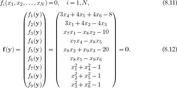
As we indicated for the single-equation Newton–Raphson method, while for our two-mass problem we can derive analytic expressions for the derivatives ∂fi/∂xj, there are 9×9 = 81 such derivatives for this (small) problem, and entering them all would be both time-consuming and error-prone. In contrast, especially for more complicated problems, it is straightforward to program a forward-difference approximation for the derivatives,
where each individual xj is varied independently since these are partial derivatives and δxj are some arbitrary changes you input. While a central-difference approximation for the derivative would be more accurate, it would also require more evaluations of the f’s, and once we find a solution it does not matter how accurate our algorithm for the derivative was.
As also discussed for the 1-D Newton–Raphson method (§7.10.1), the method can fail if the initial guess is not close enough to the zero of f (here all N of them) for the f ‘s to be approximated as linear. The backtracking technique may be applied here as well, in the present case, progressively decreasing the corrections ∆xi until |f|2 = |f 1|2 + |f2|2 + • • • + |fN|2 decreases.
8.3 Classes of Matrix Problems (Math)
It helps to remember that the rules of mathematics apply even to the world’s most powerful computers. For example, you should have problems solving equations if you have more unknowns than equations or if your equations are not linearly independent. But do not fret. While you cannot obtain a unique solution when there are not enough equations, you may still be able to map out a space of allowable solutions. At the other extreme, if you have more equations than unknowns, you have an overdetermined problem, which may not have a unique solution. An overdetermined problem is sometimes treated using data fitting in which a solution to a sufficient set of equations is found, tested on the unused equations, and then improved if needed. Not surprisingly, this latter technique is known as the linear least-squares method because it finds the best solution “on the average.”
The most basic matrix problem is the system of linear equations you have to solve for the two-mass problem:
![]()
where A is a known N × N matrix, x is an unknown vector of length N, and b is a known vector of length N. The best way to solve this equation is by Gaussian elimination or lower-upper (LU) decomposition. This yields the vector x without explicitly calculating A-1. Another, albeit slower and less robust, method is to determine the inverse of A and then form the solution by multiplying both sides of (8.19) by A-1:
Both the direct solution of (8.19) and the determination of a matrix’s inverse are standards in a matrix subroutine library.
If you have to solve the matrix equation
![]()
with x an unknown vector and λ an unknown parameter, then the direct solution (8.20) will not be of much help because the matrix b = λx contains the unknowns λ and x. Equation (8.21) is the eigenvalue problem. It is harder to solve than (8.19) because solutions exist for only certain λ values (or possibly none depending on A). We use the identity matrix to rewrite (8.21) as
![]()
and we see that multiplication by [A - λI]-1 yields the trivial solution
![]()
While the trivial solution is a bona fide solution, it is trivial. A more interesting solution requires the existence of a condition that forbids us from multiplying both sides of (8.22) by [A - λI]-1. That condition is the nonexistence of the inverse, and if you recall that Cramer’s rule for the inverse requires division by det[A - λI], it is clear that the inverse fails to exist (and in this way eigenvalues do exist) when
![]()
The λ values that satisfy this secular equation are the eigenvalues of (8.21).
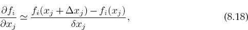
If you are interestedinonly the eigenvalues, you should look for a matrix routine that solves (8.24). To do that, first you need a subroutine to calculate the determinant of a matrix, and then a search routine to zero in on the solution of (8.24). Such routines are available in libraries. The traditional way to solve the eigenvalue problem (8.21) for both eigenvalues and eigenvectors is by diagonalization. This is equivalent to successive changes of basis vectors, each change leaving the eigenval-uesunchangedwhilecontinuallydecreasingthevaluesof theoff-diagonalelements of A. The sequence of transformations is equivalent tocontinually operating onthe original equation with a matrix U:
until one is found for which UAU-1 is diagonal:
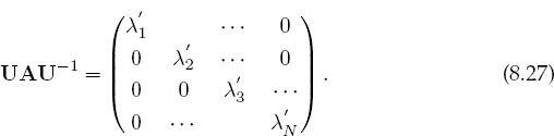
The diagonal values of UAU-1 are the eigenvalues with eigenvectors
![]()
that is, the eigenvectors are the columns of the matrix U 1. A number of routines of this type are found in subroutine libraries.
8.3.1 Practical Aspects of Matrix Computing
Many scientific programming bugs arise from the improper use of arrays.2 This may be due to the extensive use of matrices in scientific computing or to the complexity of keeping track of indices and dimensions. In any case, here are some rules of thumb to observe.
Computers are finite: Unless you are careful, your matrices will use so much memory that your computation will slow down significantly, especially if it starts to use virtual memory. As a case in point, let’s say that you store data in a 4-D array with each index having a physical dimension of 100: A[100] [100] [100] [100]. This array of (100)4 64-byte words occupies ~1 GB of memory.
Processing time: Matrix operations such as inversion require on the order of N3 steps for a square matrix of dimension N. Therefore, doubling the dimensions of a 2-D square matrix (as happens when the number of integration steps is doubled) leads to an eightfold increase in processing time.
Paging: Many operating systems have virtual memory in which disk space is used when a program runs out of RAM (see Chapter 14, “High-Performance Computing Hardware, Tuning, and Parallel Computing,” for a discussion of how computers arrange memory). This is a slow process that requires writing a full page of words to the disk. If your program is near the memory limit at which paging occurs, even a slight increase in a matrix’s dimension may lead to an order-of-magnitude increase in execution time.
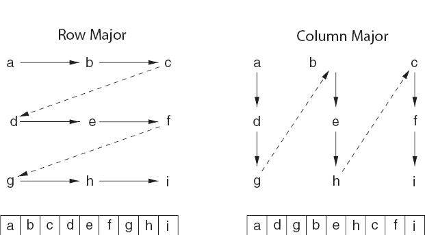
Matrix storage: While we may think of matrices as multidimensional blocks of stored numbers, the computer stores them as linear strings. For instance, a matrix a[3][3] in Java and C is stored in row-major order (Figure 8.2 left):
Figure 8.2 Left: Row-major order used for matrix storage in C and Java. Right: Column-major order used for matrix storage in Fortran. How successive matrix elements are stored in a linear fashion in memory is shown at the bottom.
while in Fortran it is stored in column-major order (Figure 8.2 right):
It is important to keep this linear storage scheme in mind in order to write proper code and to permit the mixing of Fortran and C programs.
When dealing with matrices, you have to balance the clarity of the operations being performed against the efficiency with which the computer performs them. For example, having one matrix with many indices such as V[L,Nre,Nspin,k,kp,Z,A] may be neat packaging, but it may require the computer to jump through large blocks of memory to get to the particular values needed (large strides) as you vary k, kp, and Nre. The solution would be to have several matrices such as V1[Nre,Nspin,k,kp,Z,A], V2[Nre,Nspin,k,kp,Z,A], and V3[Nre,Nspin,k,kp,Z,A].
Subscript 0: It is standard in C and Java to have array indices begin with the value 0. While this is now permitted in Fortran, the standard has been to start indices at 1. On that account, in addition to the different locations in memory due to row-major and column-major ordering, the same matrix element is referenced differently in the different languages:
Location
Java/C Element
Fortran Element
Lowest
a[0][0]
a(1,1)
a[0][1]
a(2,1)
a[1][0]
a(3,1)
a[1][1]
a(1,2)
a[2][0]
a(2,2)
Highest
a[2][1]
a(3,2)
Physical and logical dimensions: When you run a program, you issue commands such as double a[3][3] or Dimension a(3,3) that tell the compiler how much memory it needs to set aside for the array a. This is called physical memory. Sometimes you may use arrays without the full complement of values declared in the declaration statements, for example, as a test case. The amount of memory you actually use to store numbers is the matrix’s logical size.
Modern programming techniques, such as those used in Java, C, and Fortran90, permit dynamic memory allocation; that is, you may use variables as the dimension of your arrays and read in the values of the variables at run time. With these languages you should read in the sizes of your arrays at run time and thus give them the same physical and logical sizes. However, Fortran77, which is the language used for many library routines, requires the dimensions to be specified at compile time, and so the physical and logical sizes may well differ. To see why care is needed if the physical and logical sizes of the arrays differ, imagine that you declared a[3][3] but defined elements only up to a[2][2]. Then the a in storage would look like
a[1][1]’ a[1][2]’ a[1][3] a[2][1]’ a[2][2]’ a[2][3] a[3][1] a[3][2] a[3][3],
where only the elements with primes have values assigned to them. Clearly, the defined a values do not occupy sequential locations in memory, and so an algorithm processing this matrix cannot assume that the next element in memory is the next element in your array. This is the reason why subroutines from a library often need to know both the physical and logical sizes of your arrays.
Passing sizes to subprograms ©: This is needed when the logical and physical dimensions of arrays differ, as is true with some library routines but probably not with the programs you write. In cases such as those using external libraries, you must also watch that the sizes of your matrices do not exceed the bounds that have been declared in the subprograms. This may occur without an error message and probably will give you the wrong answers. In addition, if you are running a C program that calls a Fortran subroutine, you will need to pass pointers to variables and not the actual values of the variables to the Fortran subprograms (Fortran makes reference calls, which means it deals with pointers only as subprogram arguments). Here we have a program possibly running some data stored nearby:
One way to ensure size compatibility among main programs and subroutines is to declare array sizes only in your main program and then pass those sizes along to your subprograms as arguments.
Equivalence, pointers, references manipulations ©: Once upon a time computers had such limited memories that programmers conserved memory by having different variables occupy the same memory location, the theory being that this would cause no harm as long as these variables were not being used at the same time. This was done by the use of Common and Equivalence statements in Fortran and by manipulations using pointers and references in other languages. These types of manipulations are now obsolete (the bane of object-oriented programming) and can cause endless grief; do not use them unless it is a matter of “life or death”!
Say what’s happening: You decrease programming errors by using self-explanatory labels for your indices (subscripts), stating what your variables mean, and describing your storage schemes.
Tests: Always test a library routine on a small problem whose answer you know (such as the exercises in §8.3.4). Then you’ll know if you are supplying it with the right arguments and if you have all the links working.

8.3.2 Implementation: Scientific Libraries,World Wide Web
Some major scientific and mathematical libraries available include the following.
NETLIB |
A WWW metalib of free math libraries |
ScaLAPACK |
Distributed memory LAPACK |
LAPACK |
Linear Algebra Pack |
JLAPACK |
LAPACK library in Java |
SLATEC |
Comprehensive math and statistical pack |
ESSL |
Engineering and Science Subroutine Library (IBM) |
IMSL |
International Math and Statistical Libraries |
CERNLIB |
European Centre for Nuclear Research Library |
BLAS |
Basic Linear Algebra Subprograms |
JAMA |
Java Matrix Library |
NAG |
Numerical Algorithms Group (UK Labs) |
LAPACK ++ |
Linear algebra in C++ |
TNT |
C++ Template Numerical Toolkit |
GNU Scientific GSL |
Full scientific libraries in C and C++ |
Except for ESSL, IMSL, and NAG, all these libraries are in the public domain. However, even the proprietary ones are frequently available on a central computer or via an institutionwide site license. General subroutine libraries are treasures to possess because they typically contain optimized routines for almost everything you might want to do, such as
Linear algebra manipulations |
Matrix operations |
Interpolation, fitting |
Eigensystem analysis |
Signal processing |
Sorting and searching |
Solutions of linear equations |
Differential equations |
Roots, zeros, and extrema |
Random-number operations |
Statistical functions |
Numerical quadrature |
You can search the Web to find out about these libraries or to download one if it is not already on your computer. Alternatively, an excellent place to start looking for a library is Netlib, a repository of free software, documents, and databases of interest to computational scientists.
Linear Algebra Package (LAPACK) is a free, portable, modern (1990) library of Fortran77 routines for solving the most common problems in numerical linear algebra. It is designed to be efficient on a wide range of high-performance computers under the proviso that the hardware vendor has implemented an efficient set of Basic Linear Algebra Subroutines (BLAS). In contrast to LAPACK, the Sandia, Los Alamos, Air Force Weapons Laboratory Technical Exchange Committee (SLATEC) library contains general-purpose mathematical and statistical Fortran routines and is consequently more general. Nonetheless, it is not as tuned to the architecture of a particular machine as is LAPACK.
Sometimes a subroutine library supplies only Fortran routines, and this requires a C programmer to call a Fortran routine (we describe how to do that in Appendix E). In some cases, C-language routines may also be available, but they may not be optimized for a particular machine.
As an example of what may be involved in using a scientific library, consider the SLATEC library, which we recommend. The full library contains a guide, a table of contents, and documentation via comments in the source code. The subroutines are classified by the Guide to Available Mathematical Software (GAMS) system. For our masses-on-strings problem we have found the needed routines:
If you extract these routines, you will find that they need the following:
enorm.f |
j4save.f |
r1mach.f |
xerprn.f |
fdjac1.f |
r1mpyq.f |
xercnt.f |
xersve.f |
fdump.f |
qform.f |
r1updt.f |
xerhlt.f |
xgetua.f |
dogleg.f |
i1mach.f |
qrfac.f |
snsq.f |
xermsg.f |
Of particular interest in these “helper” routines, are i1mach.f, r1mach.f, and d1mach.f. They tell LAPACK the characteristic of your particular machine when the library is firstinstalled. Withoutthatknowledge,LAPACKdoes notknowwhenconvergence is obtained or what step sizes to use.
8.3.3 JAMA: Java Matrix Library
JAMA is a basic linear algebra package for Java developed at the U.S. National Institute of Science (NIST) (see reference [Jama] for documentation). We recommend it because it works well, is natural and understandable to nonexperts, is free, and helps make scientific codes more universal and portable, and because not much else is available. JAMA provides object-oriented classes that construct true Matrix objects, add and multiply matrices, solve matrix equations, and print out entire matrices in an aligned row-by-row format. JAMAis intended to serve as the standard matrix class for Java.3 Because this book uses Java for its examples, we now give some JAMA examples.
The first example is the matrix equation Ax = b for the solution of a set of linear equations with x unknown. We take A to be 3×3, x to be 3×1, and b to be 3×1:

Here the vectors and matrices are declared and created as Matrix variables, with b given random values. We then solve the 3×3 linear system of equations Ax = b with the single command Matrix x = A.solve(b) and compute the residual Ax-b with the command Residual = A.times(x).minus(b).
Our second JAMA example arises in the solution for the principal-axes system for a cube and requires us to find a coordinate system in which the inertia tensor is diagonal. This entails solving the eigenvalue problem
![]()
where I is the original inertia matrix, ω is an eigenvector, λ is an eigenvalue, and we use arrows to indicate vectors. The program JamaEigen.java in Listing 8.1 solves for the eigenvalues and vectors and produces output of the form
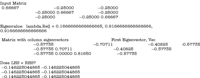
Look at JamaEigen and notice how on line 9 we first set up the array I with all the elements of the inertia tensor and then on line 10 create a matrix MatI with the same elements as the array. On line 13 the eigenvalue problem is solved with the creation of an eigenvalue object E via the JAMA command:

Listing 8.1 JamaEigen.java uses the JAMA matrix library to solve eigenvalue problems. Note that JAMA defines and manipulates the new data type (object) Matrix,which differs from an array but can be created from one.
![]()
Then on line 14 we extract (get) a vector lambdaRe of length 3 containing the three (real) eigenvalues lambdaRe[0], lambdaRe[1], lambdaRe[2]:
![]()
On line 18 we create a 3×3 matrix V containing the eigenvectors in the three columns of the matrix with the JAMA command:
![]()
which takes the eigenvector object E and gets the vectors from it. Then, on lines 22–24 we form a vector Vec (a 3×1 Matrix) containing a single eigenvector by extracting the elements from V with a get method and assigning them with a set method:
![]()

Listing 8.2 JamaFit.java performs a least-squares fit of a parabola to data using the JAMA matrix library to solve the set of linear equations ax = b.
Our final JAMAexample, JamaFit.java in Listing 8.2, demonstrates many of the features of JAMA. It arises in the context of least-squares fitting, as discussed in §8.7 where we give the equations being used to fit the parabola y(x) = b0 +b1x+b2x2 to a set of ND measured data points (yi, yi ± σi). For illustration, the equation is solved both directly and by matrix inversion, and several techniques for assigning values to JAMA’s Matrix are used.
8.3.4 Exercises for Testing Matrix Calls
Before you direct the computer to go off crunching numbers on a million elements of some matrix, it’sagood idea for you to try out your procedures on a small matrix, especially one for which you know the right answer. In this way it will take you only a short time to realize how hard it is to get the calling procedure perfectly right! Here are some exercises.
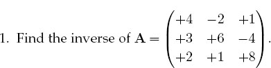
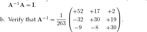
a. As a general procedure, applicable even if you do not know the analytic answer, check your inverse in both directions; that is, check that AA-1 = A-1A=I.
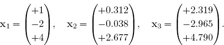
2. Consider the same matrix A as before, now used to describe three simultaneous linear equations, Ax = b, or explicitly,
Here the vector b on the RHS is assumed known, and the problem is to solve for the vector x. Use an appropriate subroutine to solve these equations for the three different x vectors appropriate to these three different b values on the RHS:

The solutions should be
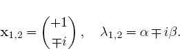
3. Consider the matrix ![]() where you are free to use any values
where you are free to use any values
you want for α and β. Use a numerical eigenproblem solver to show that the eigenvalues and eigenvectors are the complex conjugates
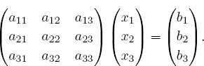
4. Use your eigenproblem solver to find the eigenvalues of the matrix

a. Verify that you obtain the eigenvalues λ1 = 5, λ2 = λ3 = -3. Notice that double roots can cause problems. In particular, there is a uniqueness prob- lemwith their eigenvectorsbecauseany combinationof these eigenvectors is also an eigenvector.
b. Verify that the eigenvector for λ1 = 5 is proportional to

c. The eigenvalue -3 corresponds to a double root. This means that the corresponding eigenvectors are degenerate, which in turn means that they are not unique. Two linearly independent ones are

In this case it’s not clear what your eigenproblem solver will give for the eigenvectors. Try to find a relationship between your computed eigenvectors with the eigenvalue -3 and these two linearly independent ones.
5. Your model of some physical system results in N = 100 coupled linear equations in N unknowns:

In many cases, the a and b values are known, so your exercise is to solve for all the x values, taking a as the Hilbert matrix and b as its first row:

![]()
8.3.5 Matrix Solution of the String Problem
We have now set up the solution to our problem of two masses on a string and have the matrix tools needed to solve it. Your problem is to check out the physical reasonableness of the solution for a variety of weights and lengths. You should check that the deduced tensions are positive and that the deduced angles correspond to a physical geometry (e.g., with a sketch). Since this is a physics-based problem, we know that the sine and cosine functions must be less than 1 in magnitude and that the tensions should be similar in magnitude to the weights of the spheres.
8.3.6 Explorations
1. See at what point your initial guess gets so bad that the computer is unable to find a physical solution.
2. A possible problem with the formalism we have just laid out is that by incorporating the identity sin2 θi + cos2 θi = 1 into the equations we may be discarding some information about the sign of sinθ or cosθ. If you look at Figure 8.1, you can observe that for some values of the weights and lengths, θ2 may turn out to be negative, yet cosθ should remain positive. We can build this condition into our equations by replacing f7 -f9 with f’s based on the form

See if this makes any difference in the solutions obtained.
2.![]() Solve the similar three-mass problem. The approach is the same, but the number of equations gets larger.
Solve the similar three-mass problem. The approach is the same, but the number of equations gets larger.
![]()
8.4 Unit II. Data Fitting
Data fitting is an art worthy of serious study by all scientists. In this unit we just scratch the surface by examining how to interpolate within a table of numbers and how to do a least-squares fit to data. We also show how to go about making a least-squares fit to nonlinear functions using some of the search techniques and subroutine libraries we have already discussed.
8.5 Fitting an Experimental Spectrum (Problem)
Problem: The cross sections measured for the resonant scatteringofaneutron from a nucleus are given in Table 8.1 along with the measurement number (index), the energy, and the experimental error. Your problem is to determine values for the cross sections at energy values lying between those measured by experiment.
You can solve this problem in a number of ways. The simplest is to numerically interpolate between the values of the experimental f(Ei) given in Table 8.1. This is direct and easy but does not account for there being experimental noise in the data. A more appropriate way to solve this problem (discussed in §8.7) is to find the best fit of a theoretical function to the data. We start with what we believe to be the “correct” theoretical description of the data,
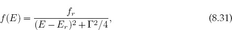
where fr,Er, and Γ are unknown parameters. We then adjust the parameters to obtain the best fit. This is a best fit in a statistical sense but in fact may not pass through all (or any) of the data points. For an easy, yet effective, introduction to statistical data analysis, we recommend [B&R 02].
These two techniques of interpolation and least-squares fitting are powerful tools that let you treat tables of numbers as if they were analytic functions and sometimes let you deduce statistically meaningful constants or conclusions from measurements. In general, you can view data fitting as global or local. In global fits,
TABLE 8.1
Experimental Values for a Scattering Cross Section g(E) as a Function of Energy

a single function in x is used to represent the entire set of numbers in a table like Table 8.1. While it may be spiritually satisfying to find a single function that passes through all the data points, if that function is not the correct function for describing the data,thefit may show nonphysical behavior (suchaslarge oscillations) between the data points. The rule of thumb is that if you must interpolate, keep it local and view global interpolations with a critical eye.
8.5.1 Lagrange Interpolation (Method)
Consider Table 8.1 as ordered data that we wish to interpolate. We call the independent variable x and its tabulated values xi(i = 1,2,…), and we assume that the dependent variable is the function g(x), with tabulated values gi = g(xi). We assume that g(x) can be approximated as a (n-1)-degree polynomial in each interval i:
Because ourfitislocal,wedonot assume that oneg(x) canfit all the datainthe table but instead use a different polynomial, that is, a different set of ai values, for each region of the table. While each polynomial is of low degree, multiple polynomials are used to span the entire table. If some care is taken, the set of polynomials so obtained will behave well enough to be used in further calculations without introducing much unwanted noise or discontinuities.
The classic interpolation formula was created by Lagrange. He figured out a closed-form one that directly fits the (n - 1)-order polynomial (8.32) to n values of the function g(x) evaluated at the points xi. The formula is written as the sum of polynomials:
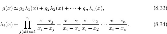
For three points, (8.33) provides a second-degree polynomial, while for eight points it gives a seventh-degree polynomial. For example, here we use a four-point Lagrange interpolation to determine a third-order polynomial that reproduces the values x1-4 = (0,1,2,4), f1-4 = (-12,-12,-24,-60):
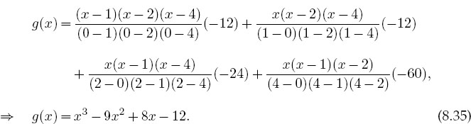
As a check we see that
![]()
If the data contain little noise, this polynomial can be used with some confidence within the range of the data, but with risk beyond the range of the data.
Notice that Lagrange interpolation makes no restriction that the points in the table be evenly spaced. As a check, it is also worth noting that the sum of the Lagrange multipliers equals one, ¿^i=1 λi = 1. Usually the Lagrange fit is made to only a small region of the table with a small value of n, even though the formula works perfectly well for fitting a high-degree polynomial to the entire table. The difference between the value of the polynomial evaluated at some x and that of the actual function is equal to the remainder

where ζ lies somewhere in the interpolation interval but is otherwise undetermined. This shows that if significant high derivatives exist in g(x), then it cannot be approximated well by a polynomial. In particular, if g(x) is a tableof experimental data, it is likely to contain noise, and then it is a bad idea to fit a curve through all the data points.
8.5.2 Lagrange Implementation and Assessment
Consider the experimental neutron scattering data in Table 8.1. The expected theoretical functional form that describes these data is (8.31), and our empirical fits to these data are shown in Figure 8.3.
1. Write a subroutinetoperform an n-point Lagrange interpolation using (8.33). Treat n as an arbitrary input parameter. (You can also do this exercise with the spline fits discussed in § 8.5.4.)
2. Use the Lagrange interpolation formula to fit the entire experimental spectrum with one polynomial. (This means that you must fit all nine data points with an eight-degree polynomial.) Then use this fit to plot the cross section in steps of 5MeV.
3. Use your graphtodeduce the resonance energyEr (your peakposition) and Γ (the full width at half-maximum). Compare your results with those predicted by our theorist friend, (Er,Γ) = (78,55) MeV.
4. A more realistic use of Lagrange interpolation is for local interpolation with a small number of points, such as three. Interpolate the preceding cross-sectionaldatain5-MeVsteps using three-point Lagrange interpolation. (Note that the end intervals may be special cases.)
![]()
This example shows how easy it is to go wrong with a high-degree-polynomial fit. Although the polynomial is guaranteed to pass through all the data points, the representation of the function away from these points can be quite unrealistic. Using a low-order interpolation formula, say, n = 2 or 3, in each interval usually eliminates the wild oscillations. If these local fits are then matched together, as we discuss in the next section, a rather continuous curve results. Nonetheless, you must recall that if the data contain errors, a curve that actually passes through them may lead you astray. We discuss how to do this properly in §8.7.
8.5.3 Explore Extrapolation
We deliberately have not discussed extrapolation of data because it can lead to serious systematic errors; the answer you get may well depend more on the function you assume than on the data you input. Add some adventure to your life and use the programs you have written to extrapolate to values outside Table 8.1. Compare your results to the theoretical Breit–Wigner shape (8.31).
![]()
8.5.4 Cubic Splines (Method)
If you tried to interpolate the resonant cross section with Lagrange interpolation, then you saw that fitting parabolas (three-point interpolation) within a table may avoid the erroneous and possibly catastrophic deviations of a high-order formula. (A two-point interpolation, which connects the points with straight lines, may not lead you far astray, but it is rarely pleasing to the eye or precise.) A sophisticated variationofann = 4 interpolation, knownascubic splines, often leadstosurprisingly eye-pleasing fits. In this approach (Figure 8.3), cubic polynomials are fit to the function in each interval, with the additional constraint that the first and second derivatives of the polynomials be continuous from one interval to the next. This continuity of slope and curvature is what makes the spline fit particularly eye-pleasing. It is analogous to what happens when you use the flexible spline drafting tool (a lead wire within a rubber sheath) from which the method draws its name.
The series of cubic polynomials obtained by spline-fitting a table of data can be integrated and differentiated and is guaranteed to have well-behaved derivatives.

Figure 8.3 Three fits to cross-section data. Short dashed line: Lagrange interpolation using an eight-degree polynomial that passes through all the data points but has nonphysical oscillations between points; solid line: cubic splines (smooth but not accurate); dashed line: Least-squares parabola fit (a best fit with a bad theory). The best approach is to do a least-squares fit of the correct theoretical function, the Breit–Wigner method (8.31).
The existence of meaningful derivatives is an important consideration. As a case in point, if the interpolated function is a potential, you can take the derivative to obtain the force. The complexity of simultaneously matching polynomials and their derivatives over all the interpolation points leads to many simultaneous linear equations to be solved. This makes splines unattractive for hand calculation, yet easyfor computers and, not surprisingly,popularinbothcalculationsandgraphics. To illustrate, the smooth curves connecting points in most “draw” programs are usually splines, as is the solid curve in Figure 8.3.
The basic approximation of splines is the representation of the function g(x) in the subinterval [xi, xi+1] with a cubic polynomial:
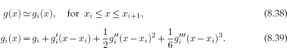
This representation makes it clear that the coefficients in the polynomial equal the values of g(x) and its first, second, and third derivatives at the tabulated points xi. Derivatives beyond the third vanish for a cubic. The computational chore is to determine these derivatives in terms of the N tabulated gi values. The matching of gi at the nodes that connect one interval to the next provides the equations
The matching of the first and second derivatives at each interval’s boundaries provides the equations
![]()
The additional equationsneededtodetermineall constantsisobtainedbymatching the third derivatives at adjacent nodes. Values for the third derivatives are found by approximating them in terms of the second derivatives:
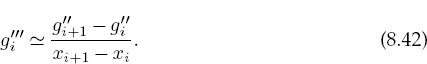
As discussed in Chapter 7, “Differentiation & Searching,” a central-difference approximation would be better than a forward-difference approximation, yet (8.42) keeps the equations simpler.
It is straightforward though complicated to solve for all the parameters in (8.39). We leave that to other reference sources [Thom 92, Pres 94]. We can see, however, that matching at the boundaries of the intervals results in only (N — 2) linear equations for N unknowns. Further input is required. It usually is taken to be the boundary conditions at the endpoints a = x and b = x, specifically, the second derivatives g’(a) and g’(b). There are several ways to determine these second derivatives:
Natural spline: Set g’(a) = g’(b) = 0; that is, permit the function to have a slope at the endpoints but no curvature. This is “natural” because the derivative vanishes for the flexible spline drafting tool (its ends being free).
Input values for g’ at the boundaries: The computer uses g’(a) to approximate g"(a). If you do not know the first derivatives, you can calculate them numerically from the table of g¿ values.
Input values for g” at the boundaries: Knowing values is of course better than approximating values, but it requires the user to input information. If the values of g” are not known, they can be approximated by applying a forward-difference approximation to the tabulated values:

8.5.4.1 CUBIC SPLINE QUADRATURE (EXPLORATION)
A powerful integration scheme is to fit an integrand with splines and then integrate the cubic polynomials analytically. If the integrand g(x) is known only at its tabulated values, then this is about as good an integration scheme as is possible; if you have the ability to calculate the function directly for arbitrary x, Gaussian quadrature may be preferable. We know that the spline fit to g in each interval is the cubic (8.39)
It is easy to integrate this to obtain the integral of g for this interval and then to sum over all intervals:
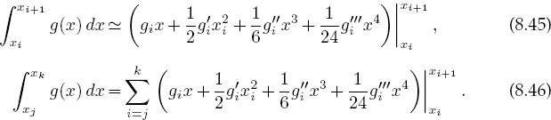
Making the intervals smaller does not necessarily increase precision, as subtractive cancellations in (8.45) may get large.
8.5.5 Spline Fit of Cross Section (Implementation)
Fitting a series of cubics to data is a little complicated to program yourself, so we recommend using a library routine. While we have found quite a few Java-based spline applications available on the internet, none seemed appropriate for interpreting a simple set of numbers. That being the case, we have adapted the splint.c and the spline.c functions from [Pres 94] to produce the SplineAppl.java program shown in Listing 8.3 (there is also an applet version on the CD (available online: http://press.princeton.edu/landau_survey/)). Your problem now is to carry out the assessment in § 8.5.2 using cubic spline interpolation rather than Lagrange interpolation.
![]()
8.6 Fitting Exponential Decay (Problem)
Figure 8.4 presents actual experimental data on the number of decays ∆N of the π meson as a function of time [Stez 73]. Notice that the time has been “binned” into ∆ t = 10-ns intervals and that the smooth curve is the theoretical exponential decay expected for very large numbers. Your problem is to deduce the lifetime τ of the π meson from these data (the tabulated lifetime of the pion is 2.6 χ 10~8 s).
8.6.1 Theory to Fit
Assume that we start with N0 particles at time t = 0 that can decay to other particles.4 If we wait a short time ∆ t, then a small number ∆N of the particles will decay spontaneously, that is, with no external influences. This decay is a stochastic process, which means that there is an element of chance involved in just when a decay will occur, and so no two experiments are expected to give exactly the same results. The basic law of nature for spontaneous decay is that the number of decays ∆N in a time interval ∆ t is proportional to the number of particles N(t) present at that time and to the time interval
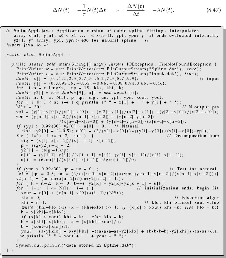
Listing 8.3 SplineAppl.java is an application version of an applet given on the CD (available online: http://press.princeton.edu/landau_survey/) that performs a cubic spline fit to data. The arrays x [] and y [] are the data to fit, and the values of the fit at Nfit points are output into the file Spline.dat.
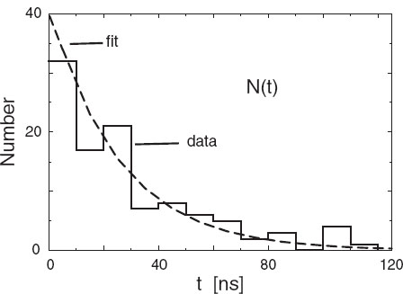
Figure 8.4 A reproduction of the experimental measurement in [Stez 73] of the number of decays of a π meson as a function of time. Measurements are made during time intervals of 10-ns length. Each “event” corresponds to a single decay.
Here τ = Ι/λ is the lifetime of the particle, with λ the rate parameter. The actual decay rate is given by the second equation in (8.47). If the number of decays AN is very small compared to the number of particles N, and if we look at vanishingly small time intervals, then the difference equation (8.47) becomes the differential equation

This differential equation has an exponential solution for the number as well as for the decay rate:
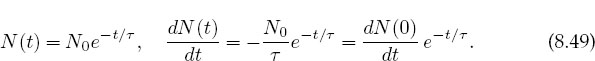
Equation (8.49) is the theoretical formula we wish to “fit” to the data in Figure 8.4. The output of such a fit is a “best value” for the lifetime τ.
8.7 Least-Squares Fitting (Method)
Books have been written and careers have been spent discussing what is meant by a “good fit” to experimental data. We cannot do justice to the subject here and refer the reader to [B&R 02, Pres 94, M&W 65, Thom 92]. However, we will emphasize three points:
1. If the data being fit contain errors, then the “best fit” in a statistical sense should not pass through all the data points.
2. If the theory is not an appropriate one for the data (e.g., the parabola in Figure 8.3), then its best fit to the data may not be a good fit at all. This is good, for it indicates that this is not the right theory.
3. Only for the simplest case of a linear least-squares fit can we write down a closed-form solution to evaluate and obtainthefit.More realisticproblems are usually solved by trial-and-error search procedures, sometimes using sophisticated subroutine libraries. However, in §8.7.6weshow howtoconduct such a nonlinear search using familiar tools.
Imagine that you have measured ND data values of the independent variable y as a function of the dependent variable x:
where ±σi is the uncertainty in the ith value of y. (For simplicity we assume that all the errors σi occur in the dependent variable, although this is hardly ever true [Thom 92]). For our problem, y is the number of decays as a function of time, and xi are the times. Our goal is to determine how well a mathematical function y = g(x) (also called a theory or a model) can describe these data. Alternatively, if the theory contains some parameters or constants, our goal can be viewed as determining the best values for these parameters. We assume that the model function g(x) contains, in addition to the functional dependence on x, an additional dependence upon MP parameters {a 1, a2,…, aMP}. Notice that the parameters {am} are not variables, in the sense of numbers read from a meter, but rather are parts of the theoretical model, such as the size of a box, the mass of a particle, or the depth of a potential well. For the exponential decay function (8.49), the parameters are the lifetime τ and the initial decay rate dN(0)/dt. We indicate this as
![]()
We use the chi-square (χ2) measure as a gauge of how well a theoretical function g reproduces data:

where the sum is over the ND experimental points (xi,yi ±σi). The definition (8.52) is such that smaller values of χ2 are better fits, with χ2 = 0 occurring if the theoretical curve went through the center of every data point. Notice also that the 1/σi2 weighting means that measurements with larger errors5 contribute less to χ2.
Least-squares fitting refers to adjusting the parameters in the theory until a minimum in χ2 is found, that is, finding a curve that produces the least value for the summed squares of the deviations of the data from the function g(x). In general, this is the best fit possible or the best way to determine the parameters in a theory. The MP parameters {am,m = 1,MP} that make χ2 an extremum are found by solving the MP equations:

More usually, the function g(x; {am}) has a sufficiently complicated dependence on the am values for (8.53) to produce MP simultaneous nonlinear equations in the am values. In these cases, solutions are found by a trial-and-error search through the MP-dimensional parameter space, as we do in §8.7.6. To be safe, when such a search is completed, you need to check that the minimum χ2 you found is global and not local. One way to do that is to repeat the search for a whole grid of starting values, and if different minima are found, to pick the one with the lowest χ2.
8.7.1 Least-Squares Fitting: Theory and Implementation
When the deviations from theory are due to random errors and when these errors are described by a Gaussian distribution, there are some useful rules of thumb to remember [B&R 02]. You know that your fit is good if the value of χ2 calculated via the definition (8.52) is approximately equal to the number of degrees of freedom χ2 ~ ND – MP, where ND is the number of data points and MP is the number of parameters in the theoretical function. If your χ2 is much less than ND – MP, it doesn’t mean that you have a “great” theory or a really precise measurement; instead, you probably have too many parameters or have assigned errors (σi values) that are too large. In fact, too small a χ2 may indicate that you are fitting the random scatter in the data rather than missing approximately one-third of the error bars, as expected for anormal distribution. If your χ2 is significantly greater than ND – MP, the theory may not be good, you may have significantly underestimated your errors, or you may have errors that are not random.
The MP simultaneous equations (8.53) can be simplified considerably if the functions g(x; {am}) depend linearly on the parameter values ai, e.g.,
![]()

Figure 8.5 Left: A linear least-squares best fit of data to a straight line. Here the deviation of theory from experiment is greater than would be expected from statistics, or in other words, a straight line is not a good theory for these data. Right: A linear least-squares best fit of different data to a parabola. Here we see that the fit misses approximately one-third of the points, as expected from the statistics for a good fit.
In this case (also known as linear regression and shown on the left in Figure 8.5) there are MP = 2 parameters, the slope a2, and the y intercept a1. Notice that while there are only two parameters to determine, there still may be an arbitrary number ND of data points to fit. Remember, a unique solution is not possible unless the number of data points is equal to or greater than the number of parameters. For this linear case, there are just two derivatives,

and after substitution, the χ2 minimization equations (8.53) can be solved [Pres 94]:

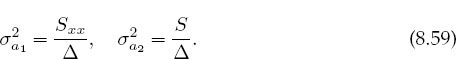
Statistics also gives you an expression for the variance or uncertainty in the deduced parameters:
This is a measure of the uncertainties in the values of the fitted parameters arising from the uncertainties σi in the measured yi values. A measure of the dependence of the parameters on each other is given by the correlation coefficient:
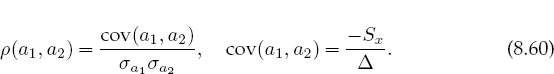
Here cov(a1,a2) is the covariance of a1 and a2 and vanishes if a1 and a2 are independent. The correlation coefficient ρ(a1,a2) lies in the range — 1 < ρ < 1, with a positive ρ indicating that the errors in a1 and a2 are likely to have the same sign, and a negative ρ indicating opposite signs.
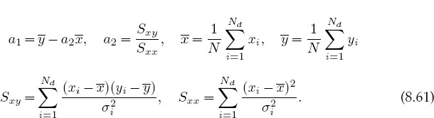
The preceding analytic solutions for the parameters are of the form found in statistics books but are not optimal for numerical calculations because subtractive cancellation can make the answers unstable. As discussed in Chapter 2, “Errors & Uncertainties in Computations,” a rearrangement of the equations can decrease this type of error. For example, [Thom 92] gives improved expressions that measure the data relative to their averages:
In JamaFit.java in Listing 8.2 and on the CD, we give a program that fits a parabola to some data. You can use it as a model for fitting a line to data, although you can use our closed-form expressions for a straight-line fit. In Fit.java on the instructor’s CD (available online: http://press.princeton.edu/landau_survey/) we give a program for fitting to the decay data.
![]()
8.7.2 Exponential Decay Fit Assessment
Fit the exponential decay law (8.49) to the data in Figure 8.4. This means finding values for τ and ∆N(0)/∆t that provide a best fit to the data and then judging how good the fit is.
1. Construct a table (∆N/∆ti, ti), for i = 1,ND from Figure 8.4. Because time was measured in bins, ti should correspond to the middle of a bin.
2. Add an estimate of the error σi to obtain a table of the form (∆N/∆ti ± σi,ti). You can estimate the errors by eye, say, by estimating how much the histogram values appear to fluctuate about a smooth curve, or you can take σi ~ Vevents. (This last approximation is reasonable for large numbers, which this is not.)
3. In the limit of very large numbers, we would expect a plot of ln dN/dt versus t to be a straight line:
This means that if we treat ln ∆N(t)/∆t as the dependent variable and time ∆ t as the independent variable, we can use our linear fit results. Plot ln ∆N/∆t versus ∆t.
4. Make a least-squares fit of a straight line to your data and use it to determine the lifetime τ of the π meson. Compare your deduction to the tabulated lifetime of 2.6 χ 10~8 s and comment on the difference.
5. Plot your best fit on the same graph as the data and comment on the agreement.
6. Deduce the goodness of fit of your straight line and the approximate error in your deduced lifetime. Do these agree with what your “eye” tells you?
![]()
8.7.3 Exercise: Fitting Heat Flow
The table below gives the temperature T along a metal rod whose ends are kept at a fixed constant temperature. The temperature is a function of the distance x along the rod.
xi (cm) |
1.0 |
2.0 |
3.0 |
4.0 |
5.0 |
6.0 |
7.0 |
8.0 |
9.0 |
Ti (C) |
14.6 |
18.5 |
36.6 |
30.8 |
59.2 |
60.1 |
62.2 |
79.4 |
99.9 |
1. Plot the data to verify the appropriateness of a linear relation
![]()
2. Because you are not given the errors for each measurement, assume that the least significant figure has been rounded off and so σ > 0.05. Use that to compute a least-squares straight-line fit to these data.
3. Plot your best a + bx on the curve with the data.
4. After fitting the data, compute the variance and compare it to the deviation of your fit from the data. Verify that about one-third of the points miss the σ error band (that’s what is expected for a normal distribution of errors).
5. Use your computed variance to determine the χ2 of the fit. Comment on the value obtained.
6. Determine the variances σα and σ and check whether it makes sense to use them as the errors in the deduced values for a and b.
![]()
8.7.4 Linear Quadratic Fit (Extension)
As indicated earlier, as long as the function being fitted depends linearly on the unknown parameters ai, the condition of minimum χ2 leads to a set of simultaneous linear equations for the a’s that can be solved on the computer using matrix techniques. To illustrate, suppose we want to fit the quadratic polynomial
to the experimental measurements (xi, yi, i = 1, ND) (Figure 8.5 right). Because this g(x) is linear in all the parameters ai, we can still make a linear fit even though x is raised to the second power. [However, if we tried to a fit a function of the form g(x) = (a1 +a2x) exp(-a3 x) to the data, then we would not be able to make a linear fit because one of the a’s appears in the exponent.]
The best fit of this quadratic to the data is obtained by applying the minimum χ2 condition (8.53) for Mp = 3 parameters and ND (still arbitrary) data points. A solution represents the maximum likelihood that the deduced parameters provide a correct description of the data for the theoretical function g(x). Equation (8.53) leads to the three simultaneous equations for a1, a2, and a3:

Note: Because the derivatives are independent of the parameters (the a’s), the a dependence arises only from the term in square brackets in the sums, and because that term has only a linear dependence on the a’s, these equations are linear equations in the a’s.
Exercise: Show that after some rearrangement, (8.64)–(8.66) can be written as

Here the definitions of the S’s are simple extensions of those used in (8.56)–(8.58) and are programmed in JamaFit.java shown in Listing 8.2. After placing the three parameters into a vector a and the three RHS terms in (8.67) into a vector S, these equations assume the matrix form:

This is the exactly the matrix problem we solved in §8.3.3 with the code JamaFit.java given in Listing 8.2. The solution for the parameter vector a is obtained by solving the matrix equations. Although for 3×3 matrices we can write out the solution in closed form, for larger problems the numerical solution requires matrix methods.
8.7.5 Linear Quadratic Fit Assessment
1. Fit the quadratic (8.63) to the following data sets [given as (x1, y1), (x2, y2),…]. In each case indicate the values found for the a’s, the number of degrees of freedom, and the value of χ2.
a. (0, 1)
b. (0, 1), (1, 3)
c. (0, 1), (1, 3), (2, 7)
d. (0, 1), (1, 3), (2, 7), (3, 15)
2. Find a fit to the last set of data to the function
![]()
Hint: A judicious change of variables will permit you to convert this to a linear fit. Does a minimum χ2 still have meaning here?
![]()
8.7.6 Nonlinear Fit of the Breit–Wigner Formula to a Cross Section
Problem: Remember how we started Unit II of this chapter by interpolating the values in Table 8.1, which gave the experimental cross section Σ as a function of energy. Although we did not use it, we also gave the theory describing these data, namely, the Breit–Wigner resonance formula (8.31):

Your problem here is to determine what values for the parameters Er,fr, and Γ in (8.70) provide the best fit to the data in Table 8.1.
Because (8.70) is not a linear function of the parameters (Er,Σ0,Γ), the three equations that result from minimizing χ2 are not linear equations and so cannot be solved by the techniques of linear algebra (matrix methods). However, in our study of the masses on a string problem in Unit I, we showed how to use the Newton–Raphson algorithm to search for solutions of simultaneous nonlinear equations. That technique involved expansion of the equations about the previous guess to obtain a set of linear equations and then solving the linear equations with the matrix libraries. We now use this same combination of fitting, trial-and-error searching, and matrix algebra to conduct a nonlinear least-squares fit of (8.70) to the data in Table 8.1.
Recollect that the condition for a best fit is to find values of the MP parameters am in the theory g(x, am) that minimize χ2 = 5^i[(yi — gi )/σi]2. This leads to the MP equations (8.53) to solve

To find the form of these equations appropriate to our problem, we rewrite our theory function (8.70) in the notation of (8.71):

The three derivatives required in (8.71) are then

Substitution of these derivatives into the best-fit condition (8.71) yields three simultaneous equations in a1, a2, and a3 that we need to solve in order to fit the ND = 9 data points (xi, yi) in Table 8.1:

Even without the substitution of (8.70) for g(x, a), it is clear that these three equations depend on the a’s in a nonlinear fashion. That’s okay because in §8.2.2 we derived the N-dimensional Newton–Raphson search for the roots of
where we have made the change of variable yi —> ai for the present problem. We use that same formalism here for the N = 3 equations (8.74) by writing them as

Because fr = a is the peak value of the cross section, ER = a2 is the energy at which the peak occurs, andΓ = 2v/ai is the full width of the peak at half-maximum, good guesses for the a’s can be extracted from a graph of the data. To obtain the nine derivatives of the three f’s with respect to the three unknown a’s, we use two nested loops over i and j, along with the forward-difference approximation for the derivative

where ∆aj corresponds to a small, say <1%, change in the parameter value.
8.7.6.1 NONLINEAR FIT IMPLEMENTATION
Use the Newton–Raphson algorithm as outlined in §8.7.6 to conduct a nonlinear search for the best-fit parameters of the Breit-Wigner theory (8.70) to the data in Table 8.1. Compare the deduced values of (fr,ER, Γ) to that obtained by inspection of the graph. The program Newton_Jama2.java on the instructor’s CD (available online: http://press.princeton.edu/landau_survey/) solves this problem.
![]()
1 Althoughwe prize the book [Pres 94] and whatithas accomplished,wecannot recommend taking subroutines from it. They are neither optimized nor documented for easy, standalone use, whereas the subroutine libraries recommended in this chapter are.
2 Even a vector V (N) is called an array, albeit a 1-D one.
3 A sibling matrix package, Jampack [Jama] has also been developed at NIST and at the University of Maryland, and it works for complex matrices as well.
4 Spontaneous decay is discussed further and simulated in § 5.5.
5 If you are not given the errors, you can guess them on the basis of the apparent deviation of the data from a smooth curve, or you can weigh all points equally by setting σi ≡ 1 and continue with the fitting.