7

Differentiation & Searching

In this chapter we add two more tools to our computational toolbox: numerical differentiation and trial-and-error searching. In Unit I we derive the forward-difference, central-difference, and extrapolated-difference methods for differentiation. They will be used throughout the book, especially for partial differential equations. In Unit II we devise ways to search for solutions to nonlinear equations by trial and error and apply our new-found numerical differentiation tools there. Although trial-and-error searching may not sound very precise, it is in fact widely used to solve problems where analytic solutions do not exist or are not practical. In Chapter 8, “Solving Systems of Equations with Matrices; Data Fitting,” we extend these search and differentiation techniques to the solution of simultaneous equations using matrix techniques. In Chapter 9, “Differential Equation Applications,” we combine trial-and-error searching with the solution of ordinary differential equations to solve the quantum eigenvalue problem.

7.1  Unit I. Numerical Differentiation

Problem: Figure 7.1 shows the trajectory of a projectile with air resistance. The dots indicate the times t at which measurements were made and tabulated. Your problem is to determine the velocity dy/dt = y’ as a function of time. Note that since there is realistic air resistance present, there is no analytic function to differentiate, only this table of numbers.

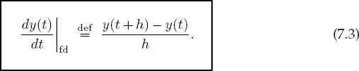
You probably did rather well in your first calculus course and feel competent at taking derivatives. However, you may not ever have taken derivatives of a table of numbers using the elementary definition

In fact, even a computer runs into errors with this kind of limit because it is wrought with subtractive cancellation; the computer’s finite word length causes the numerator to fluctuate between 0 and the machine precision em as the denominator approaches zero.

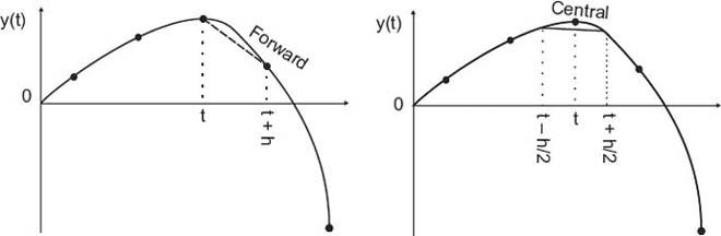
Figure 7.1 Forward-difference approximation (slanted dashed line) and central-difference approximation (horizontal line) for the numerical first derivative at point t. The central difference is seen to be more accurate. (The trajectory is that of a projectile with air resistance.)

7.2  Forward Difference (Algorithm)

The most direct method for numerical differentiation starts by expanding a function in a Taylor series to obtain its value a small step h away:

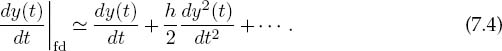
We obtain the forward-difference derivative algorithm by solving (7.2) for y’(t):

An approximation for the error follows from substituting the Taylor series:

You can think of this approximation as using two points to represent the function by a straight line in the interval from x to x + h (Figure 7.1 left).

The approximation (7.3) has an error proportional to h (unless the heavens look down upon you kindly and make y” vanish). We can make the approximation error smaller by making h smaller, yet precision will be lost through the subtractive cancellation on the left-hand side (LHS) of (7.3) for too small an h. To see how the forward-difference algorithm works, let y(t) = a + bt2. The exact derivative is y’ = 2bt, while the computed derivative is

This clearly becomes a good approximation only for small h(h <C 2t).

7.3  Central Difference (Algorithm)

An improved approximation to the derivative starts with the basic definition (7.1) or geometrically as shown in Figure 7.1 on the right. Now, rather than making a single step of h forward, we form a central difference by stepping forward half a step and backward half a step:

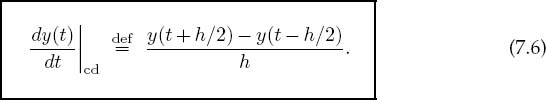
We estimate the error in the central-difference algorithm by substituting the Taylor series for y(t ± h/2) into (7.6):

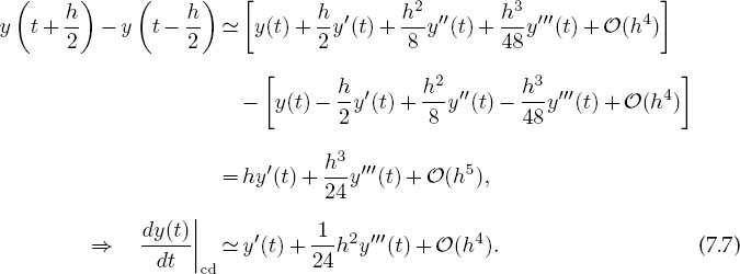
The important difference between this algorithm and the forward difference from (7.3) is that when y(t – h/2) is subtracted from y(t + h/2), all terms containing an even power of h in the two Taylor series cancel. This make the central-difference algorithm accurate to order h2 (h3 before division by h), while the forward difference is accurate only to order h. If the y(t) is smooth, that is, if y’"h2/24 <C y"h/2, then you can expect the central-difference error to be smaller. If we now return to our parabola example (7.5), we will see that the central difference gives the exact derivative independent of h:

7.4  Extrapolated Difference (Method)

Because a differentiation rule based on keeping a certain number of terms in a Taylor series also provides an expression for the error (the terms not included), we can reduce the theoretical error further by forming a combination of algorithms whose summed errors extrapolate to zero. One algorithm is the central-difference algorithm(7.6)usingahalf-stepbackandahalf-step forward. Thesecond algorithm is another central-difference approximation using quarter-steps:

A combination of the two eliminates both the quadratic and linear error terms:

Here (7.10) is the extended-difference algorithm, (7.11) gives its error, and Dc¿ represents the central-difference algorithm. If h = 0.4 and y^ 1, then there will be only one place of round-off error and the truncation error will be approximately machine precision em; this is the best you can hope for.

When working with these and similar higher-order methods, it is important to remember that while they may work as designed for well-behaved functions, they may fail badly for functions containing noise, as may data from computations or measurements. If noise is evident, it may be better to first smooth the data or fit them with some analytic function using the techniques of Chapter 8, “Solving Systems of Equations with Matrices; Data Fitting,” and then differentiate.

7.5  Error Analysis (Assessment)

The approximation errors in numerical differentiation decrease with decreasing step size h, while round-off errors increase with decreasing step size (you have to take more steps and do more calculations). Remember from our discussion in Chapter 2, “Errors & Uncertainties in Computations,” that the best approximation occurs for an h that makes the total error _approx + _ro a minimum, and that as a rough guide this occurs when e_ro — _approx.

We have already estimated the approximation error in numerical differentiation rules by making a Taylor series expansion of y (x + h). The approximation error with the forward-difference algorithm (7.3) is O(h), while that with the central-difference algorithm (7.7) is O (h2):

To obtain a rough estimate of the round-off error, we observe that differentiation essentially subtracts the value of a function at argument x from that of the same function at argument x + h and then divides by h: y’ — [y(t + h) — y(t)]/h. As h is made continually smaller, we eventually reach the round-off error limit where y(t + h) and y(t) differ by just machine precision em:

Consequently, round-off and approximation errors become equal when

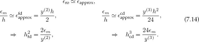
We take y’ ~ y⁽²⁾ y⁽³⁾ (which may be crude in general, though not bad for et or cost) and assume double precision, em ~ 10-¹⁵:

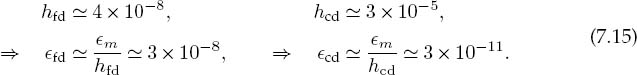
This may seem backward because the better algorithm leads to a larger h value. It is not. The ability to use a larger h means that the error in the central-difference method is about 1000 times smaller than the error in the forward-difference method.

We give a full program Diff.java on the instructor’s disk, yet the programming for numerical differentiation is so simple that we need give only the lines

7.6  Second Derivatives (Problem)

Let’s say that you have measured the position y(t) versus time for a particle (Figure 7.1). Your problem now is to determine the force on the particle. Newton’s second law tells us that force and acceleration are linearly related:

where F is the force, m is the particle’s mass, and a is the acceleration. So if we can determine the acceleration a(t) = d²y/dt² from the y(t) values, we can determine the force.

The concerns we expressed about errors in first derivatives are even more valid for second derivatives where additional subtractions may lead to additional cancellations. Let’s look again at the central-difference method:

This algorithm gives the derivative at t by moving forward and backward from t by h/2. We take the second derivative d²y/dt² to be the central difference of the first derivative:

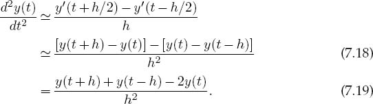
As we did for first derivatives, we determine the second derivative at t by evaluating the function in the region surrounding t. Although the form (7.19) is more compact and requires fewer steps than (7.18), it may increase subtractive cancellation by first storing the “large” number y(t + h)+ y(t — h) and then subtracting another large number 2y(t) from it. We ask you to explore this difference as an exercise.

7.6.1  Second-Derivative Assessment

Write a program to calculate the second derivative of cost using the central- difference algorithms (7.18) and (7.19). Test it over four cycles. Start with h ~ π/10 and keep reducing h until you reach machine precision.

7.7  Unit II. Trial-and-Error Searching

Many computer techniques are well-defined sets of procedures leading to definite outcomes. In contrast, some computational techniques are trial-and-error algorithms in which decisions on what steps to follow are made based on the current values of variables, and the program quits only when it thinks it has solved the problem. (We already did some of this when we summed a power series until the terms became small.) Writing this type of program is usually interesting because we must foresee how to have the computer act intelligently in all possible situations, and running them is very much like an experiment in which it is hard to predict what the computer will come up with.

7.8  Quantum States in a Square Well (Problem)

Probably the most standard problem in quantum mechanics¹ is to solve for the energies of a particle of mass m bound within a 1-D square well of radius a:

As shown in quantum mechanics texts [Gott 66], the energies of the bound states E = -EB < 0 within this well are solutions of the transcendental equations

where even and odd refer to the symmetry of the wave function. Here we have chosen units such that h = 1, 2m = 1, a = 1, and V0 = 10. Your problem is to

7.9  Trial-and-Error Roots via the Bisection Algorithm

Trial-and-error root finding looks for a value of x at which

where the 0 on the right-hand side (RHS) is conventional (an equation such as 10 sin x = 3x3 can easily be written as 10 sin x – 3x3 = 0). The search procedure starts with a guessed value for x, substitutes that guess into f (x) (the “trial”), and then sees how far the LHS is from zero (the “error”). The program then changes x based on the error and tries out the new guess in f(x). The procedure continues until f (x) 0 to some desired level of precision, until the changes in x are insignificant, or until it appears that progress is not being made.

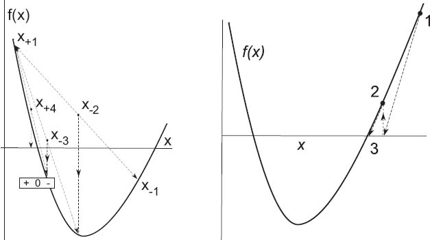
Figure 7.2 A graphical representation of the steps involved in solving for a zero of f (x) using the bisection algorithm (left) and the Newton–Raphson method (right). The bisection algorithm takes the midpoint of the interval as the new guess for x, and so each step reduces the interval size by one-half. The Newton–Raphson method takes the new guess as the zero of the line tangent to f(x) at the old guess. Four steps are shown for the bisection algorithm, but only two for the more rapidly convergent Newton–Raphson method.

The most elementary trial-and-error technique is the bisection algorithm. It is reliable but slow. If you know some interval in which f(x) changes sign, then the bisection algorithm will always converge to the root by finding progressively smaller and smaller intervals in which the zero occurs. Other techniques, such as the Newton–Raphson method we describe next, may converge more quickly, but if the initial guess is not close, it may become unstable and fail completely.

The basis of the bisection algorithm is shown on the left in Figure 7.2. We start with two values of x between which we know a zero occurs. (You can determine these by making a graph or by stepping through different x values and looking for a sign change.) To be specific, let us say that f (x) is negative at x_ and positive at x+:

(Note that it may well be that x- > x₊ if the function changes from positive to negative as x increases.) Thus we start with the interval x₊ ≤ x ≤ x- within which we know a zero occurs. The algorithm (given on the CD (available online: http://press.princeton.edu/landau_survey/) as Bisection.java) then picks the new x as the bisection of the interval and selects as its new interval the half in which the sign change occurs:

This process continues until the value of f(x) is less than a predefined level of precision or until a predefined (large) number of subdivisions occurs.

The example in Figure 7.2 on the left shows the first interval extending from x- = x₊₁ to x₊ = x-₁. We then bisect that interval at x, and since f(x) < 0 at the midpoint, we set x- ≡ x-₂ = x and label it x-₂ to indicate the second step. We then use x₊₂ ≡ x₊₁ and x-₂ as the next interval and continue the process. We see that only x- changes for the first three steps in this example, but that for the fourth step x₊ finally changes. The changes then become too small for us to show.

7.9.1  Bisection Algorithm Implementation

7.10  Newton–Raphson Searching (A Faster Algorithm)

The Newton–Raphson algorithm finds approximate roots of the equation

more quickly than the bisection method. As we see graphically in Figure 7.2 on the right, this algorithm is the equivalent of drawing a straight line f (x) mx + b tangent to the curve at an x value for which f (x) 0 and then using the intercept of the line with the x axis at x = -b/m as an improved guess for the root. If the “curve” were a straight line, the answer would be exact; otherwise, it is a good approximation if the guess is close enough to the root for f (x) to be nearly linear. The process continues until some set level of precision is reached. If a guess is in a region where f (x) is nearly linear (Figure 7.2), then the convergence is much more rapid than for the bisection algorithm.

The analytic formulation of the Newton–Raphson algorithm starts with an old guess xQ and expresses a new guess x as a correction ∆x to the old guess:

We next expand the known function f(x) in a Taylor series around x₀ and keep only the linear terms:

We then determine the correction ∆x by calculating the point at which this linear approximation to f (x) crosses the x axis:

The procedure is repeated starting at the improvedxuntil some set level of precision is obtained.

The Newton–Raphson algorithm (7.29) requires evaluation of the derivative df/dx at each value of x₀. In many cases you may have an analytic expression for the derivative and can build it into the algorithm. However, especially for more complicated problems, it is simpler and less error-prone to use a numerical forward-difference approximation to the derivative:²

where δx is some small change in x that you just chose [different from the ∆ used for searching in (7.29)]. While a central-difference approximation for the derivative would be more accurate, it would require additional evaluations of the f’s, and once you find a zero, it does not matter how you got there. On the CD (available online: http://press.princeton.edu/landau_survey/) we give the

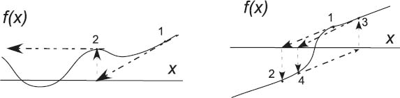
Figure 7.3 Two examples of how the Newton–Raphson algorithm may fail if the initial guess is not in the region where f(x) can be approximated by a straight line. Left: A guess lands at a local minimum/maximum,that is, a place where the derivative vanishes,and so the next guess ends up at x = ∞. Right: The search has fallen into an infinite loop. Backtracking would help here.

programs Newton_cd.java (also Listing 7.1) and Newton_fd.java,which implement the derivative both ways.

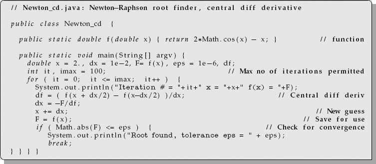
Listing 7.1 Newton cd.java uses the Newton–Raphson method to search for a zero of the function f(x). A central-difference approximation is used to determine df/dx.

7.10.1  Newton–Raphson Algorithm with Backtracking

Two examples of possible problems with the Newton–Raphson algorithm are shown in Figure 7.3. On the left we see a case where the search takes us to an x value where the function has a local minimum or maximum, that is, where df/dx = 0. Because ∆x = —f/f’, this leads to a horizontal tangent (division by zero), and so the next guess is x = oo, from where it is hard to return. When this happens, you need to start your search with a different guess and pray that you do not fall into this trap again. In cases where the correction is very large but maybe not infinite, you may want to try backtracking (described below) and hope that by taking a smaller step you will not get into as much trouble.

In Figure 7.3 on the right we see a case where a search falls into an infinite loop surrounding the zero without ever getting there. Asolution to this problem is called backtracking. As the name implies, in cases where the new guess x0 +∆x leads to an increase in the magnitude of the function, |f(x0 +∆x)|2 > | f(x0)|2, you should backtrack somewhat and try a smaller guess, say, x ₀ + ∆x/2. If the magnitude of f still increases, then you just need to backtrack some more, say, by trying x ₀ + ∆x/4 as your next guess, and so forth. Because you know that the tangent line leads to a local decrease in | f |, eventually an acceptable small enough step should be found.

The problem in both these cases is that the initial guesses were not close enough to the regions where f (x) is approximately linear. So again, a good plot may help produce a good first guess. Alternatively, you may want to start your search with the bisection algorithm and then switch to the faster Newton–Raphson algorithm when you get closer to the zero.

7.10.2  Newton–Raphson Algorithm Implementation

1 We solve this same problem in §9.9 using an approach that is applicable to almost any potential and which also provides the wave functions. The approach of this section works only for the eigenenergies of a square well.

2 We discuss numerical differentiation in Chapter 7, “Differentiation & Searching.”