
14
High-Performance Computing Hardware, Tuning, and Parallel Computing
In this chapter and in Appendix D we discuss a number of topics associated with high-performance computing (HPC). If history can be our guide, today’s HPC hardware and software will be on desktop machines a decade from now. In Unit I we discuss the theory of a high-performance computer’s memory and central processor design. In Unit II we examine parallel computers. In Appendix D we extend Unit II by giving a detailed tutorial on use of the message-passing interface (MPI) package, while a tutorial on an earlier package, Parallel virtual machine (PVM), is provided on the CD (available online: http://press.princeton.edu/landau_survey/). In Unit III we discuss some techniques for writing programs that are optimized for HPC hardware, such as virtual memory and cache. By running the short implementations given in Unit III, you will experiment with your computer’s memory and experience some of the concerns, techniques, rewards, and shortcomings of HPC.
HPC is a broad subject, and our presentation is brief and given from a practitioner’s point of view. The text [Quinn 04] surveys parallel computing and MPI from a computer science point of view. References on parallel computing include [Sterl 99, Quinn 04, Pan 96, VdeV 94, Fox 94]. References on MPI include Web resources [MPI, MPI2, MPImis] and the texts [Quinn 04, Pach 97, Lusk 99]. More recent developments, such as programming for multicore computers, cell computers, and field-programmable gate accelerators, will be discussed in future books.
14.1 Unit I. High-Performance Computers (CS)
By definition, supercomputers are the fastest and most powerful computers available, and at this instant, the term “supercomputers” almost always refers to parallel machines.They are the superstars of the high-performance class of computers. Unix workstations and modern personal computers (PCs), which are small enough in size and cost to be used by a small group or an individual, yet powerful enough for large-scale scientific and engineering applications, can also be high-performance computers. We define high-performance computers as machines with a good balance among the following major elements:
• Multistaged (pipelined) functional units.
• Multiple central processing units (CPUs) (parallel machines).
• Multiple cores.
• Fast central registers.
• Very large, fast memories.
• Very fast communication among functional units.
• Vector, video, or array processors.
• Software that integrates the above effectively.
As a simple example, it makes little sense to have a CPU of incredibly high speed coupled to a memory system and software that cannot keep up with it (the present state of affairs).
14.2 Memory Hierarchy
An idealized model of computer architecture is a CPU sequentially executing a stream of instructions and reading from a continuous block of memory. To illustrate, in Figure 14.1 we see a vector A [] and an array M [] [] loaded in memory and about to be processed. The real world is more complicated than this. First, matrices are not stored in blocks but rather in linear order. For instance, in Fortran it is in column-major order:
M(1,1) M(2,1) M(3,1) M(1,2) M(2,2) M(3,2) M(1,3) M(2,3) M(3,3),
while in Java and C it is in row-major order:
M(0,0) M(0,1) M(0,2) M(1,0) M(1,1) M(1,2) M(2,0) M(2,1) M(2,2).
Second, the values for the matrix elements may not even be in the same physical place. Some may be in RAM, some on the disk, some in cache, and some in the CPU. To give some of these words more meaning, in Figures 14.2 and 14.3 we show simple models of the memory architecture of a high-performance computer. This hierarchical arrangement arises from an effort to balance speed and cost with fast, expensive memory supplemented by slow, less expensive memory. The memory architecture may include the following elements:
CPU: Central processing unit, the fastest part of the computer. The CPU consists of a number of very-high-speed memory units called registers containing the instructions sent to the hardware to do things like fetch, store, and operate on data. There are usually separate registers for instructions, addresses, and operands (current data). In many cases the CPU also contains some specialized parts for accelerating the processing of floating-point numbers.
Cache (high-speed buffer): A small, very fast bit of memory that holds instructions, addresses, and data in their passage between the very fast CPU registers and the slower RAM. This is seen in the next level down the pyramid in Figure 14.3. The main memory is also called dynamic RAM (DRAM), while the cache is called static RAM (SRAM). If the cache is used properly, it eliminates the need for the CPU to wait for data to be fetched from memory.
Cache and data lines: The data transferred to and from the cache or CPU are grouped into cache lines or data lines. The time it takes to bring data from memory into the cache is called latency.

Figure 14.1 The logical arrangement of the CPU and memory showing a Fortran array A(N) and matrix M(N, N) loaded into memory.
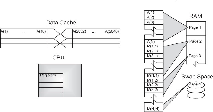
Figure 14.2 The elements of a computer’s memory architecture in the process of handling matrix storage.

Figure 14.3 Typical memory hierarchy for a single-processor, high-performance computer (B = bytes, K, M, G, T = kilo, mega, giga, tera).
RAM: Random-access memory or central memory is in the middle memory in the hierarchy in Figure 14.3. RAM can be accessed directly, that is, in random order, and it can be accessed quickly, that is, without mechanical devices. It is where your program resides while it is being processed.
Pages: Central memory is organized into pages, which are blocks of memory of fixed length. The operating system labels and organizes its memory pages much like we do the pages of a book; they are numbered and kept track of with a table of contents. Typical page sizes are from 4 to 16 kB.
Hard disk: Finally, at the bottom of the memory pyramid is permanent storage on magnetic disks or optical devices. Although disks are very slow compared to RAM, they can store vast amounts of data and sometimes compensate for their slower speeds by using a cache of their own, the paging storage controller.
Virtual memory: True to its name, this is a part of memory you will not find in our figures because it is virtual. It acts like RAM but resides on the disk.
When we speak of fast and slow memory we are using a time scale set by the clock in the CPU. To be specific, if your computer has a clock speed or cycle time of 1 ns, this means that it could perform a billion operations per second if it could get its hands on the needed data quickly enough (typically, more than 10 cycles are needed to execute a single instruction). While it usually takes 1 cycle to transfer data from the cache to the CPU, the other memories are much slower, and so you can speed your program up by not having the CPU wait for transfers among different levels of memory. Compilers try to do this for you, but their success is affected by your programming style.

Figure 14.4 Multitasking of four programs in memory at one time in which the programs are executed in round-robin order.
As shown in Figure 14.2 for our example, virtual memory permits your program to use more pages of memory than can physically fit into RAM at one time. A combination of operating system and hardware maps this virtual memory into pages with typical lengths of 4–16 KB. Pages not currently in use are stored in the slower memory on the hard disk and brought into fast memory only when needed. The separate memory location for this switching is known as swap space (Figure 14.2). Observe that when the application accesses the memory location for M[i][j], the number of the page of memory holding this address is determined by the computer, and the location of M[i][j] within this page is also determined. A page fault occurs if the needed page resides on disk rather than in RAM. In this case the entire page must be read into memory while the least recently used page in RAM is swapped onto the disk. Thanks to virtual memory, it is possible to run programs on small computers that otherwise would require larger machines (or extensive reprogramming). The price you pay for virtual memory is an order-of-magnitude slowdown of your program’s speed when virtual memory is actually invoked. But this may be cheap compared to the time you would have to spend to rewrite your program so it fits into RAM or the money you would have to spend to buy a computer with enough RAM for your problem.
Virtual memory also allows multitasking, the simultaneous loading into memory of more programs than can physically fit into RAM (Figure 14.4). Although the ensuing switching among applications uses computing cycles, by avoiding long waits while an application is loaded into memory, multitasking increases the total throughout and permits an improved computing environment for users. For example, it is multitasking that permits a windows system to provide us with multiple windows. Even though each window application uses a fair amount of memory, only the single application currently receiving input must actually reside in memory; the rest are paged out to disk. This explains why you may notice a slight delay when switching to an idle window; the pages for the now active program are being placed into RAM and the least used application still in memory is simultaneously being paged out.
TABLE 14.1
Computation of c = (a+ b)/(d ∗f)

14.3 The Central Processing Unit
How does the CPU get to be so fast? Often, it employs prefetching and pipelining; that is, it has the ability to prepare for the next instruction before the current one has finished. It is like an assembly line or a bucket brigade in which the person filling the buckets at one end of the line does not wait for each bucket to arrive at the other end before filling another bucket. In the same way a processor fetches, reads, and decodes an instruction while another instruction is executing. Consequently, even though it may take more than one cycle to perform some operations, it is possible for data to be entering and leaving the CPU on each cycle. To illustrate, Table 14.1 indicates how the operation c = (a+b)/(d∗f)is handled. Here the pipelined arithmetic unitsA1andA2are simultaneously doing their jobs of fetching and operating on operands, yet arithmetic unit A3 must wait for the first two units to complete their tasks before it has something to do (during which time the other two sit idle).
14.4 CPU Design: Reduced Instruction Set Computer
Reduced instruction set computer (RISC) architecture (also called superscalar) is a design philosophy for CPUs developed for high-performance computers and now used broadly. It increases the arithmetic speed of the CPU by decreasing the number of instructions the CPU must follow. To understand RISC we contrast it with complex instruction set computer (CISC), architecture. In the late 1970s, processor designers began to take advantage of very-large-scale integration (VLSI) which allowed the placement of hundreds of thousands of devices on a single CPU chip. Much of the space on these early chips was dedicated to microcode programs written by chip designers and containing machine language instructions that set the operating characteristics of the computer. There were more than 1000 instructions available, and many were similar to higher-level programming languages like Pascal and Forth. The price paid for the large number of complex instructions was slow speed, with a typical instruction taking more than 10 clock cycles. Furthermore, a 1975 study by Alexander and Wortman of the XLP compiler of the IBM System/360 showed that about 30 low-level instructions accounted for 99% of the use with only 10 of these instructions accounting for 80% of the use.
The RISC philosophy is to have just a small number of instructions available at the chip level but to have the regular programmer’s high level-language, such as Fortran or C, translate them into efficient machine instructions for a particular computer’s architecture. This simpler scheme is cheaper to design and produce, lets the processor run faster, and uses the space saved on the chip by cutting down on microcode to increase arithmetic power. Specifically, RISC increases the number of internal CPU registers, thus making it possible to obtain longer pipelines (cache) for the data flow, a significantly lower probability of memory conflict, and some instruction-level parallelism.
The theory behind this philosophy for RISC design is the simple equation describing the execution time of a program:
Here “CPU time” is the time required by a program, “no. instructions” is the total number of machine-level instructions the program requires (sometimes called the path length), “cycles/instruction” is the number of CPU clock cycles each instruction requires, and “cycle time” is the actual time it takes for one CPU cycle. After viewing (14.1) we can understand the CISC philosophy, which tries to reduce CPU time by reducing no. instructions, as well as the RISC philosophy, which tries to reduce CPU time by reducing cycles/instruction (preferably to one). For RISC to achieve an increase in performance requires a greater decrease in cycle time and cycles/instruction than the increase in the number of instructions.
In summary, the elements of RISC are the following.
Single-cycle execution for most machine-level instructions.
Small instruction set of less than 100 instructions.
Register-based instructions operating on values in registers, with memory access confined to load and store to and from registers.
Many registers, usually more than 32.
Pipelining, that is, concurrent processing of several instructions.
High-level compilers to improve performance.
14.5 CPU Design: Multiple-Core Processors
The year preceding the publication of this book has seen a rapid increase in the inclusion of dual-core, or even quad-core, chips as the computational engine of computers.As seen in Figure 14.5, a dual-core chip has two CPUs in one integrated circuit with a shared interconnect and a shared level-2 cache. This type of configuration with two or more identical processors connected to a single shared main memory is called symmetric multiprocessing, or SMP. It is likely that by the time you read this book, 16-core or greater chips will be available.
Although multicore chips were designed for game playing and single precision, they should also be useful in scientific computing if new tools, algorithms, and programming methods are employed. These chips attain more speed with less heat and more energy efficiency than single-core chips, whose heat generation limits them to clock speeds of less than 4 GHz. In contrast to multiple single-core chips, multicore chips use fewer transistors per CPU and are thus simpler to make and cooler to run.
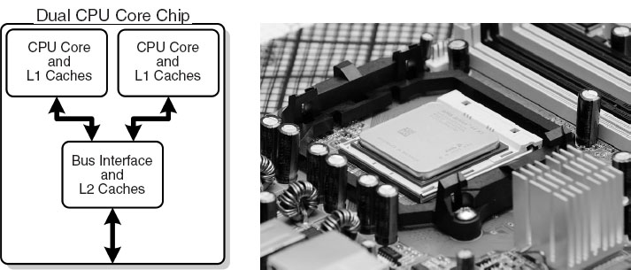
Figure 14.5 Left: A generic view of the Intel core-2 dual-core processor,with CPU-local level-1 caches and a shared,on-die level-2 cache (courtesy of D. Schmitz). Right: The AMD Athlon 64 X2 3600 dual-core CPU (Wikimedia Commons).
Parallelism is built into a multicore chip because each core can run a different task. However, since the cores usually share the same communication channel and level-2 cache, there is the possibility of a communication bottleneck if both CPUs use the bus at the same time. Usually the user need not worry about this, but the writers of compilers and software must so that your code will run in parallel. As indicated in our MPI tutorial in Appendix D, modern Intel compilers make use of each multiple core and even have MPI treat each core as a separate processor.
14.6 CPU Design: Vector Processor
Often the most demanding part of a scientific computation involves matrix operations. On a classic (von Neumann) scalar computer, the addition of two vectors of physical length 99 to form a third ultimately requires 99 sequential additions (Table 14.2). There is actually much behind-the-scenes work here. For each element i there is the fetch of a(i) from its location in memory, the fetch of b(i) from its location in memory, the addition of the numerical values of these two elements in a CPU register, and the storage in memory of the sum in c(i). This fetching uses up time and is wasteful in the sense that the computer is being told again and again to do the same thing.
When we speak of a computer doing vector processing, we mean that there are hardware components that perform mathematical operations on entire rows or columns of matrices as opposed to individual elements. (This hardware can also handle single-subscripted matrices, that is, mathematical vectors.) In the vector processing of [A]+[B] = [C], the successive fetching of and addition of the elements A and B are grouped together and overlaid, and Z ![]() 64-256 elements (the section size) are processed with one command, as seen in Table 14.3. Depending on the array size, this method may speed up the processing of vectors by a factor of about 10. If all Z elements were truly processed in the same step, then the speedup would be ~ 64-256.
64-256 elements (the section size) are processed with one command, as seen in Table 14.3. Depending on the array size, this method may speed up the processing of vectors by a factor of about 10. If all Z elements were truly processed in the same step, then the speedup would be ~ 64-256.
TABLE 14.2
Computation of Matrix [C] = [A] + [B]
Step 1 |
Step 2 |
… |
Step 99 |
c(1) = a(1) +b(1) |
c(2) = a(2) +b(2) |
… |
c(99) = a(99) + b(99) |
TABLE 14.3
Vector Processing of Matrix [A] + [B] = [C]
Step 1 |
Step 2 |
Step 3 |
… |
Step Z |
c(1) = a(1) +b(1) |
||||
c(2) = a(2) +b(2) |
||||
c(3) = a(3) + b(3) |
||||
… |
||||
c(Z) = a(Z)+b(Z) |
Vector processing probably had its heyday during the time when computer manufacturers produced large mainframe computers designed for the scientific and military communities. These computers had proprietary hardware and software and were often so expensive that only corporate or military laboratories could afford them. While the Unix and then PC revolutions have nearly eliminated these large vector machines, some do exist, as well as PCs that use vector processing in their video cards. Who is to say what the future holds in store?
14.7 Unit II. Parallel Computing
There is little question that advances in the hardware for parallel computing are impressive. Unfortunately, the software that accompanies the hardware often seems stuck in the 1960s. In our view, message passing has too many details for application scientists to worry about and requires coding at a much, or more, elementary level than we prefer. However, the increasing occurrence of clusters in which the nodes are symmetric multiprocessors has led to the development of sophisticated compilers that follow simpler programming models; for example, partitioned global address space compilers such as Co-Array Fortran, Unified Parallel C, and Titanium. In these approaches the programmer views a global array of data and then manipulates these data as if they were contiguous. Of course the data really are distributed, but the software takes care of that outside the programmer’s view. Although the program may not be as efficient a use of the processors as hand coding, it is a lot easier, and as the number of processors becomes very large, one can live with a greater degree of inefficiency. In any case, if each node of the computer has a number of processors with a shared memory and there are a number of nodes, then some type of a hybrid programming model will be needed.
Problem: Start with the program you wrote to generate the bifurcation plot for bug dynamics in Chapter 12, “Discrete & Continuous Nonlinear Dynamics,” and modify it so that different ranges for the growth parameter µ are computed simultaneously on multiple CPUs. Although this small a problem is not worth investing your time in to obtain a shorter turnaround time, it is worth investing your time into it gain some experience in parallel computing. In general, parallel computing holds the promise of permitting you to obtain faster results, to solve bigger problems, to run simulations at finer resolutions, or to model physical phenomena more realistically; but it takes some work to accomplish this.
14.8 Parallel Semantics (Theory)
We saw earlier that many of the tasks undertaken by a high-performance computer are run in parallel by making use of internal structures such as pipelined and segmented CPUs, hierarchical memory, and separate I/O processors. While these tasks are run “in parallel,” the modern use of parallel computing or parallelism denotes applying multiple processors to a single problem [Quinn 04]. It is a computing environment in which some number of CPUs are running asynchronously and communicating with each other in order to exchange intermediate results and coordinate their activities.
For instance, consider matrix multiplication in terms of its elements:
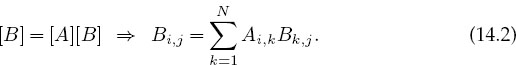
Because the computation of Bi,j for particular values of i and j is independent of the computation of all the other values, each Bi,j can be computed in parallel, or each row or column of [B] can be computed in parallel. However, because Bk,j on the RHS of (14.2) must be the “old” values that existed before the matrix multiplication, some communication among the parallel processors is required to ensure that they do not store the “new” values of Bk,j before all the multiplications are complete. This [B] = [A][B] multiplication is an example of data dependency, in which the data elements used in the computation depend on the order in which they are used. In contrast, the matrix multiplication [C] = [A][B] is a data parallel operation in which the data can be used in any order. So already we see the importance of communication, synchronization, and understanding of the mathematics behind an algorithm for parallel computation.
The processors in a parallel computer are placed at the nodes of a communication network. Each node may contain one CPU or a small number of CPUs, and the communication network may be internal to or external to the computer. One way of categorizing parallel computers is by the approach they employ in handling instructions and data. From this viewpoint there are three types of machines:
• Single-instruction, single-data (SISD): These are the classic (von Neumann) serial computers executing a single instruction on a single data stream before the next instruction and next data stream are encountered.
• Single-instruction, multiple-data (SIMD): Here instructions are processed from a single stream, but the instructions act concurrently on multiple data elements. Generally the nodes are simple and relatively slow but are large in number.
• Multiple instructions, multiple data (MIMD): In this category each processor runs independently of the others with independent instructions and data. These are the types of machines that employ message-passing packages, such as MPI,to communicate among processors. They may be a collection of work-stations linked via a network, or more integrated machines with thousands of processors on internal boards, such as the Blue Gene computer described in §14.13. These computers, which do not have a shared memory space, are also called multicomputers. Although these types of computers are some of the most difficult to program, their low cost and effectiveness for certain classes of problems have led to their being the dominant type of parallel computer at present.
The running of independent programs on a parallel computer is similar to the multitasking feature used by Unix and PCs.In multitasking (Figure 14.6 left) several independent programs reside in the computer’s memory simultaneously and share the processing time in a round robin or priority order. On a SISD computer, only one program runs at a single time, but if other programs are in memory, then it does not take long to switch to them. In multiprocessing (Figure 14.6 right) these jobs may all run at the same time, either in different parts of memory or in the memory of different computers. Clearly, multiprocessing becomes complicated if separate processors are operating on different parts of the same program because then synchronization and load balance (keeping all the processors equally busy) are concerns.

Figure 14.6 Left: Multitasking of four programs in memory at one time. On a SISD computer the programs are executed in round robin order. Right: Four programs in the four separate memories of a MIMD computer.
In addition to instructions and data streams, another way of categorizing parallel computation is by granularity. A grain is defined as a measure of the computational work to be done, more specifically, the ratio of computation work to communication work.
• Coarse-grain parallel: Separate programs running on separate computer systems with the systems coupled via a conventional communication network. An illustration is six Linux PCs sharing the same files across a network but with a different central memory system for each PC. Each computer can be operating on a different, independent part of one problem at the same time.
• Medium-grain parallel: Several processors executing (possibly different) programs simultaneously while accessing a common memory. The processors are usually placed on a common bus (communication channel) and communicate with each other through the memory system. Medium-grain programs have different, independent, parallel subroutines running on different processors. Because the compilers are seldom smart enough to figure out which parts of the program to run where, the user must include the multitasking routines in the program.1
• Fine-grain parallel: As the granularity decreases and the number of nodes increases, there is an increased requirement for fast communication among the nodes. For this reason fine-grain systems tend to be custom-designed machines. The communication may be via a central bus or via shared memory for a small number of nodes, or through some form of high-speed network for massively parallel machines. In the latter case, the compiler divides the work among the processing nodes. For example, different for loops of a program may be run on different nodes.
14.9 Distributed Memory Programming
An approach to concurrent processing that, because it is built from commodity PCs, has gained dominant acceptance for coarse- and medium-grain systems is distributed memory. In it, each processor has its own memory and the processors exchange data among themselves through a high-speed switch and network. The data exchanged or passed among processors have encoded to and from addresses and are called messages. The clusters of PCs or workstations that constitute a Beowulf 2 are examples of distributed memory computers (Figure 14.7). The unifying characteristic of a cluster is the integration of highly replicated compute and communication components into a single system, with each node still able to operate independently. In a Beowulf cluster, the components are commodity ones designed for a general market, as are the communication network and its high-speed switch (special interconnects are used by major commercial manufacturers, but they do not come cheaply). Note: A group of computers connected by a network may also be called a cluster but unless they are designed for parallel processing, with the same type of processor used repeatedly and with only a limited number of processors (the front end) onto which users may log in, they are not usually called a Beowulf.
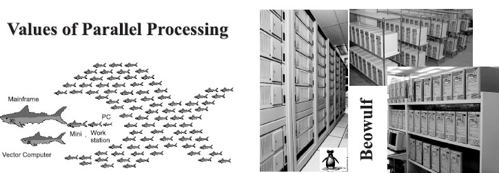
Figure 14.7 Two views of modern parallel computing (courtesy of Yuefan Deng).
The literature contains frequent arguments concerning the differences among clusters, commodity clusters, Beowulfs, constellations, massively parallel systems, and so forth [Dong 05]. Even though we recognize that there are major differences between the clusters on the top 500 list of computers and the ones that a university researcher may set up in his or her lab, we will not distinguish these fine points in the introductory materials we present here.
For a message-passing program to be successful, the data must be divided among nodes so that, at least for a while, each node has all the data it needs to run an independent subtask. When a program begins execution, data are sent to all the nodes. When all the nodes have completed their subtasks, they exchange data again in order for each node to have a complete new set of data to perform the next subtask. This repeated cycle of data exchange followed by processing continues until the full task is completed. Message-passing MIMD programs are also single-program, multiple-data programs, which means that the programmer writes a single program that is executed on all the nodes. Often a separate host program, which starts the programs on the nodes, reads the input files and organizes the output.
14.10 Parallel Performance
Imagine a cafeteria line in which all the servers appear to be working hard and fast yet the ketchup dispenser has some relish partially blocking its output and so everyone in line must wait for the ketchup lovers up front to ruin their food before moving on. This is an example of the slowest step in a complex process determining the overall rate. An analogous situation holds for parallel processing, where the “relish” may be the issuing and communicating of instructions. Because the computation cannot advance until all the instructions have been received, this one step may slow down or stop the entire process.
As we soon will demonstrate, the speedup of a program will not be significant unless you can get ∼90% of it to run in parallel, and even then most of the speedup will probably be obtained with only a small number of processors. This means that you need to have a computationally intense problem to make parallelization worthwhile, and that is one of the reasons why some proponents of parallel computers with thousands of processors suggest that you not apply the new machines to old problems but rather look for new problems that are both big enough and well-suited for massively parallel processing to make the effort worthwhile.
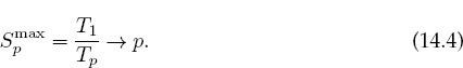
The equation describing the effect on speedup of the balance between serial and parallel parts of a program is known as Amdahl’s law [Amd 67, Quinn 04]. Let
The maximum speedup Sp attainable with parallel processing is thus
This limit is never met for a number of reasons: Some of the program is serial, data and memory conflicts occur, communication and synchronization of the processors take time, and it is rare to attain a perfect load balance among all the processors. For the moment we ignore these complications and concentrate on how the serial part of the code affects the speedup. Let f be the fraction of the program that potentially may run on multiple processors. The fraction 1−f of the code that cannot be run in parallel must be run via serial processing and thus takes time:
![]()
The time Tp spent on the p parallel processors is related to Ts by
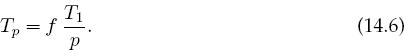
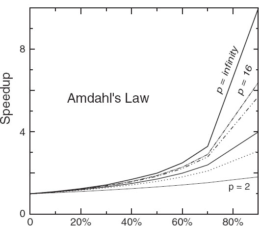
Figure 14.8 The theoretical speedup of a program as a function of the fraction of the program that potentially may be run in parallel. The different curves correspond to different numbers of processors.
That being so, the speedup Sp as a function of f and the number of processors is
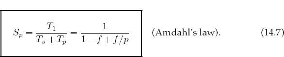
Some theoretical speedups are shown in Figure 14.8 for different numbers p of processors. Clearly the speedup will not be significant enough to be worth the trouble unless most of the code is run in parallel (this is where the 90% of your inparallel figure comes from). Even an infinite number of processors cannot increase the speed of running the serial parts of the code, and so it runs at one processor speed. In practice this means many problems are limited to a small number of processors and that often for realistic applications only 10%–20% of the computer’s peak performance may be obtained.
14.10.1 Communication Overhead
As discouraging as Amdahl’s law may seem, it actually overestimates speedup because it ignores the overhead for parallel computation. Here we look at communication overhead. Assume a completely parallel code so that its speedup is
The denominator assumes that it takes no time for the processors to communicate. However, it take a finite time, called latency, to get data out of memory and into the cache or onto the communication network. When we add in this latency, as well as other times that make up the communication time Tc, the speedup decreases to
For the speedup to be unaffected by communication time, we need to have
This means that as you keep increasing the number of processors p, at some point the time spent on computation T1/p must equal the time Tc needed for communication, and adding more processors leads to greater execution time as the processors wait around more to communicate. This is another limit, then, on the maximum number of processors that may be used on any one problem, as well as on the effectiveness of increasing processor speed without a commensurate increase in communication speed.
The continual and dramatic increases in CPU speed, along with the widespread adoption of computer clusters, is leading to a changing view as to how to judge the speed of an algorithm. Specifically, the slowest step in a process is usually the rate-determining step, and the increasing speed of CPUs means that this slowest step is more and more often access to or communication among processors. Such being the case, while the number of computational steps is still important for determining an algorithm’s speed, the number and amount of memory access and interprocessor communication must also be mixed into the formula. This is currently an active area of research in algorithm development.
14.11 Parallelization Strategy
A typical organization of a program for both serial and parallel tasks is
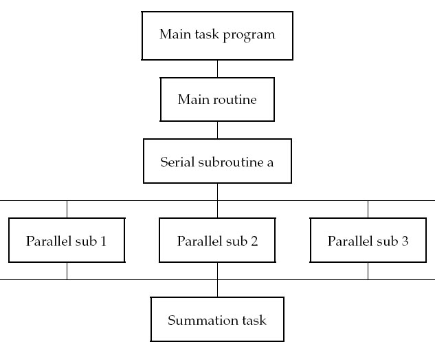
The user organizes the work into units called tasks, with each task assigning work (threads) to a processor. The main task controls the overall execution as well as the subtasks that run independent parts of the program (called parallel subroutines, slaves, guests, or subtasks). These parallel subroutines can be distinctive subprograms, multiple copies of the same subprogram, or even for loops.
It is the programmer’s responsibility to ensure that the breakup of a code into parallel subroutines is mathematically and scientifically valid and is an equivalent formulation of the original program. As a case in point, if the most intensive part of a program is the evaluation of a large Hamiltonian matrix, you may want to evaluate each rowon a different processor. Consequently, the key to parallel programming is to identify the parts of the program that may benefit from parallel execution. To do that the programmer should understand the program’s data structures (discussed below), know in what order the steps in the computation must be performed, and know how to coordinate the results generated by different processors.
The programmer helps speed up the execution by keeping many processors simultaneously busy and by avoiding storage conflicts among different parallel subprograms. You do this load balancing by dividing your program into subtasks of approximately equal numerical intensity that will run simultaneously on different processors. The rule of thumb is to make the task with the largest granularity (workload) dominant by forcing it to execute first and to keep all the processors busy by having the number of tasks an integer multiple of the number of processors. This is not always possible.
The individual parallel threads can have shared or local data. The shared data may be used by all the machines, while the local data are private to only one thread. To avoid storage conflicts, design your program so that parallel subtasks use data that are independent of the data in the main task and in other parallel tasks. This means that these data should not be modified or even examined by different tasks simultaneously. In organizing these multiple tasks, reduce communication overhead costs by limiting communication and synchronization. These costs tend to be high for fine-grain programming where much coordination is necessary. However, do not eliminate communications that are necessary to ensure the scientific or mathematical validity of the results; bad science can do harm!
14.12 Practical Aspects of Message Passing for MIMD
It makes sense to run only the most numerically intensive codes on parallel machines. Frequently these are very large programs assembled over a number of years or decades by a number of people. It should come as no surprise, then, that the programming languages for parallel machines are primarily Fortran 90, which has explicit structures for the compiler to parallelize, and C. (We have not attained good speedup with Java in parallel and therefore do not recommend it for parallel computing.) Effective parallel programming becomes more challenging as the number of processors increases. Computer scientists suggest that it is best not to attempt to modify a serial code but instead to rewrite it from scratch using algorithms and subroutine libraries best suited to parallel architecture. However, this may involve months or years of work, and surveys find that ∼70% of computational scientists revise existing codes [Pan 96].
Most parallel computations at present are done on a multiple-instruction, multiple-data computers via message passing. In Appendix D we give a tutorial on the use of MPI, the most common message-passing interface. Here we outline some practical concerns based on user experience [Dong 05, Pan 96].
Parallelism carries a price tag: There is a steep learning curve requiring intensive effort. Failures may occur for a variety of reasons, especially because parallel environments tend to change often and get “locked up” by a programming error. In addition, with multiple computers and multiple operating systems involved, the familiar techniques for debugging may not be effective.
Preconditions for parallelism: If your program is run thousands of times between changes, with execution time in days, and you must significantly increase the resolution of the output or study more complex systems, then parallelism is worth considering. Otherwise, and to the extent of the difference, parallelizing a code may not be worth the time investment.
The problem affects parallelism: You must analyze your problem in terms of how and when data are used, how much computation is required for each use, and the type of problem architecture:
• Perfectly parallel: The same application is run simultaneously on different data sets, with the calculation for each data set independent (e.g., running multiple versions of a Monte Carlo simulation, each with different seeds, or analyzing data from independent detectors). In this case it would be straightforward to parallelize with a respectable performance to be expected.
• Fully synchronous: The same operation applied in parallel to multiple parts of the same data set, with some waiting necessary (e.g., determining positions and velocities of particles simultaneously in a molecular dynamics simulation). Significant effort is required, and unless you balance the computational intensity, the speedup may not be worth the effort.
• Loosely synchronous: Different processors do small pieces of the computation but with intermittent data sharing (e.g., diffusion of groundwater from one location to another). In this case it would be difficult to parallelize and probably not worth the effort.
• Pipeline parallel: Data from earlier steps processed by later steps, with some overlapping of processing possible (e.g., processing data into images and then into animations). Much work may be involved, and unless you balance the computational intensity, the speedup may not be worth the effort.
14.12.1 High-Level View of Message Passing
Although it is true that parallel computing programs may become very complicated, the basic ideas are quite simple. All you need is a regular programming language like C or Fortran, plus four communication statements:3
send: One processor sends a message to the network. It is not necessary to indicate who will receive the message, but it must have a name.
receive: One processor receives a message from the network. This processor does not have to know who sent the message, but it has to know the message’s name.
myid: An integer that uniquely identifies each processor.
numnodes: An integer giving the total number of nodes in the system.
Once you have made the decision to run your program on a computer cluster, you will have to learn the specifics of a message-passing system such as MPI (Appendix D). Here we give a broader view. When you write a message-passing program, you intersperse calls to the message-passing library with your regular Fortran or C program. The basic steps are
1. Submit your job from the command line or a job control system.
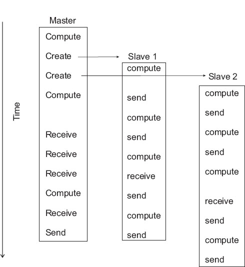
Figure 14.9 A master process and two slave processes passing messages. Notice how this program has more sends than receives and consequently may lead to results that depend on order of execution, or may even lock up.
2. Have your job start additional processes.
3. Have these processes exchange data and coordinate their activities.
4. Collect these data and have the processes stop themselves.
We show this graphically in Figure 14.9 where at the top we see a master process create two slave processes and then assign work for them to do (arrows). The processes then communicate with each other via message passing, output their data to files, and finally terminate.
What can go wrong: Figure 14.9 also illustrates some of the difficulties:
• The programmer is responsible for getting the processes to cooperate and for dividing the work correctly.
• The programmer is responsible for ensuring that the processes have the correct data to process and that the data are distributed equitably.
• The commands are at a lower level than those of a compiled language, and this introduces more details for you to worry about.
• Because multiple computers and multiple operating systems are involved, the user may not receive or understand the error messages produced.
• It is possible for messages to be sent or received not in the planned order.
• A race condition may occur in which the program results depend upon the specific ordering of messages. There is no guarantee that slave 1 will get its work done before slave 2, even though slave 1 may have started working earlier (Figure 14.9).
• Note in Figure 14.9 how different processors must wait for signals from other processors; this is clearly a waste of computer time and a potential for problems.
• Processes may deadlock, that is, wait for a message that never arrives.
14.13 Example of a Supercomputer: IBM Blue Gene/L
Whatever figures we give to describe the latest supercomputer will be obsolete by the time you read them. Nevertheless, for the sake of completeness and to set the scale for the present, we do it anyway. At the time of this writing, the fastest computer, in some aggregate sense, is the IBM Blue Gene series [Gara 05]. The name reflects its origin in a computer originally intended for gene research that is now sold as a general-purpose supercomputer (after approximately $600 million in development costs).
A building-block view of Blue Gene is given in Figure 14.10. In many ways this is a computer built by committee, with compromises made in order to balance cost, cooling, computing speed, use of existing technologies, communication speed, and so forth. As a case in point, the CPUs have dual cores, with one for computing and the other for communication. This reflects the importance of communication for distributed-memory computing (there are both on- and off-chip distributed memories). And while the CPU is fast at 5.6 GFLOPs, there are faster ones available, but they would generate so much heat that it would not be possible to obtain the extreme scalability up to 216 = 65,536 dual-processor nodes. The next objective is to balance a low cost/performance ratio with a high performance/ watt ratio.
Observe that at the lowest level Blue Gene contains two CPUs (dual cores) on a chip, with two chips on a card, with 16 cards on a board, with 32 boards in a cabinet, and up to 64 cabinets for a grand total of 65,536 CPUs (Figure 14.10). And if a way can be found to make all these chips work together for the common good on a single problem, they would turn out a peak performance of 360 ×1012 floating- point operations per second (360 tFLOPs). Each processor runs a Linux operating system (imagine what the cost in both time and money would be for Windows!) and utilizes the hardware by running a distributed memory MPI with C, C++, and Fortran90 compilers; this is not yet a good place for Java.
Blue Gene has three separate communication networks (Figure 14.11). At the heart of the memory system is a 64×32×32 3-D torus that connects all the memory blocks; Figure 14.11a shows the torus for 2×2×2 memory blocks. The links are made by special link chips that also compute; they provide both direct neighbor–neighbor communications as well as cut through communication across the network. The result of this sophisticated network is that there is approximately the same effective bandwidth and latencies (response times) between all nodes, yet in order to obtain high speed, it is necessary to keep communication local. For node-to-node communication a rate of 1.4 Gb/s = 1/10-9 s = 1 ns is obtained.

Figure 14.10 The building blocks of Blue Gene (adapted from [Gara 05]).

Figure 14.11 (a) A 3-D torus connecting 2×2×2 memory blocks. (b) The global collective memory system. (c) The control and GB-Ethernet memory system (adapted from [Gara 05]).
The latency ranges from 100 ns for 1 hop, to 6.4 µs for 64 hops between processors. The collective network in Figure 14.11b is used to communicate with all the processors simultaneously, what is known as a broadcast, and does so at 4 b/cycle. Finally, the control and gigabit ethernet network (Figure 14.11c) is used for I/O to communicate with the switch (the hardware communication center) and with ethernet devices. Its total capacity is greater than 1 tb (= 1012)/s.
The computing heart of Blue Gene is its integrated circuit and the associated memory system (Figure 14.12). This is essentially an entire computer system on a chip containing, among other things,
• two PowerPC 440s with attached floating-point units (for rapid processing of floating-point numbers); one CPU is for computing, and one is for I/O.
• a RISC architecture CPU with seven stages, three pipelines, and 32-b, 64-way associative cache lines,
• variable memory page size,
• embedded dynamic memory controllers,
• a gigabit ethernet adapter,
• a total of 512 MB/node (32 tB when summed over nodes),
• level-1 (L1) cache of 32 kB, L2 cache of 2 kB, and L3 cache of 4 MB.
14.14 Unit III. HPC Program Optimization
The type of optimization often associated with high-performance or numerically intensive computing is one in which sections of a program are rewritten and reorganized in order to increase the program’s speed. The overall value of doing this, especially as computers have become so fast and so available, is often a subject of controversy between computer scientists and computational scientists. Both camps agree that using the optimization options of compilers is a good idea. However, computational scientists tend to run large codes with large amounts of data in order to solve real-world problems and often believe that you cannot rely on the compiler to do all the optimization, especially when you end up with time on your hands waiting for the computer to finish executing your program. Here are some entertaining, yet insightful, views [Har 96] reflecting the conclusions of those who have reflected upon this issue:
More computing sins are committed in the name of efficiency (without necessarily achieving it) than for any other single reason—including blind stupidity.
— W.A. Wulf
We should forget about small efficiencies, say about 97% of the time: premature optimization is the root of all evil.
— Donald Knuth
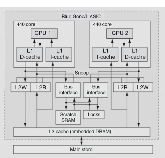
Figure 14.12 The single-node memory system (adapted from [Gara 05]).
The best is the enemy of the good.
—Voltaire
Rule 1: Do not do it.
Rule 2 (for experts only): Do not do it yet.
Do not optimize as you go: Write your program without regard to possible optimizations, concentrating instead on making sure that the code is clean, correct, and understandable. If it’s too big or too slow when you’ve finished, then you can consider optimizing it.
Remember the 80/20 rule: In many fields you can get 80% of the result with 20% of the effort (also called the 90/10 rule—it depends on who you talk to). Whenever you’re about to optimize code, use profiling to find out where that 80% of execution time is going, so you know where to concentrate your effort.
Always run “before” and “after” benchmarks: How else will you know that your optimizations actually made a difference? If your optimized code turns out to be only slightly faster or smaller than the original version, undo your changes and go back to the original, clear code.
Use the right algorithms and data structures:Do not use an O(n2) DFT algorithm to do a Fourier transform of a thousand elements when there’s an O(nlog n) FFT available. Similarly, do not store a thousand items in an array that requires an O(n) search when you could use an O(log n) binary tree or an O(1) hash table.
14.14.1 Programming for Virtual Memory (Method)
While paging makes little appear big, you pay a price because your program’s run time increases with each page fault. If your program does not fit into RAM all at once, it will run significantly slower. If virtual memory is shared among multiple programs that run simultaneously, they all can’t have the entire RAM at once, and so there will be memory access conflicts, in which case the performance of all the programs will suffer. The basic rules for programming for virtual memory are as follows.
1. Do not waste your time worrying about reducing the amount of memory used (the working set size) unless your program is large. In that case, take a global view of your entire program and optimize those parts that contain the largest arrays.
2. Avoid page faults by organizing your programs to successively perform their calculations on subsets of data, each fitting completely into RAM.
3. Avoid simultaneous calculations in the same program to avoid competition for memory and consequent page faults. Complete each major calculation before starting another.
4. Group data elements close together in memory blocks if they are going to be used together in calculations.
14.14.2 Optimizing Programs; Java versus Fortran/C
Many of the optimization techniques developed for Fortran and C are also relevant for Java applications. Yet while Java is a good language for scientific programming and is the most universal and portable of all languages, at present Java code runs slower than Fortran or C code and does not work well if you use MPI for parallel computing (see Appendix D). In part, this is a consequence of the Fortran and C compilers having been around longer and thereby having been better refined to get the most out of a computer’s hardware, and in part this is also a consequence of Java being designed for portability and not speed. Since modern computers are so fast, whether a program takes 1s or 3s usually does not matter much, especially in comparison to the hours or days of your time that it might take to modify a program for different computers. However, you may want to convert the code to C (whose command structure is very similar to that of Java) if you are running a computation that takes hours or days to complete and will be doing it many times.
Especially when asked to, Fortran and C compilers look at your entire code as a single entity and rewrite it for you so that it runs faster. (The rewriting is at a fairly basic level, so there’s not much use in your studying the compiler’s output as a way of improving your programming skills.) In particular, Fortran and C compilers are very careful in accessing arrays in memory. They also are careful to keep the cache lines full so as notto keep the CPU waiting with nothing to do. There is no fundamental reason why a program written in Java cannot be compiled to produce an highly efficient code, and indeed such compilers are being developed and becoming available. However,such code is optimized for a particular computer architecture and so is not portable. In contrast, the byte code (.class file) produced by Java is designed to be interpreted or recompiled by the Java Virtual Machine (just another program). When you change from Unix to Windows, for example, the Java Virtual Machine program changes, but the byte code is the same. This is the essence of Java’s portability.
In order to improve the performance of Java, many computers and browsers run a Just-in-Time (JIT) Java compiler. If a JIT is present, the Java Virtual Machine feeds your byte code Prog.class to the JIT so that it can be recompiled into native code explicitly tailored to the machine you are using. Although there is an extra step involved here, the total time it takes to run your program is usually 10–30 times faster with a JIT as compared to line-by-line interpretation. Because the JIT is an integral part of the Java Virtual Machine on each operating system, this usually happens automatically.
In the experiments below you will investigate techniques to optimize both Fortran and Java programs and to compare the speeds of both languages for the same computation. If you run your Java code on a variety of machines (easy to do with Java), you should also be able to compare the speed of one computer to that of another. Note that a knowledge of Fortran is not required for these exercises.
14.14.2.1 GOOD AND BAD VIRTUAL MEMORY USE (EXPERIMENT)
To see the effect of using virtual memory, run these simple pseudocode examples on your computer (Listings 14.1–14.4). Use a command such as time to measure the time used for each example. These examples call functions force12 and force21.You should write these functions and make them have significant memory requirements for both local and global variables.

Listing 14.1 BAD program, too simultaneous.
You see (Listing 14.1) that each iteration of the for loop requires the data and code for all the functions as well as access to all the elements of the matrices and arrays. The working set size of this calculation is the sum of the sizes of the arrays f12(N,N), f21(N,N), and pion(N) plus the sums of the sizes of the functions force12 and force21.
A better way to perform the same calculation is to break it into separate components (Listing 14.2):

Listing 14.2 GOOD program, separate loops.
Here the separate calculations are independent and the working set size, that is, the amount of memory used, is reduced. However, you do pay the additional overhead costs associated with creating extra for loops. Because the working set size of the first for loop is the sum of the sizes of the arrays f12(N, N) and pion(N), and of the function force12, we have approximately half the previous size. The size of the last for loop is the sum of the sizes for the two arrays. The working set size of the entire program is the larger of the working set sizes for the different for loops.
As an example of the need to group data elements close together in memory or common blocks if they are going to be used together in calculations, consider the following code (Listing 14.3):
![]()
Listing 14.3 BAD Program, discontinuous memory.
Here the variables zed, ylt, and part are used in the same calculations and are adjacent in memory because the programmer grouped them together in Common (global variables). Later, when the programmer realized that the array med2 was needed, it was tacked onto the end of Common. All the data comprising the variables zed, ylt, and part fit onto one page, but the med2 variable is on a different page because the large array zpart2(50000) separates it from the other variables. In fact, the system may be forced to make the entire 4-kB page available in order to fetch the 72 B of data in med2. While it is difficult for a Fortran or C programmer to ensure the placement of variables within page boundaries, you will improve your chances by grouping data elements together (Listing 14.4):

Listing 14.4 GOOD program, continuous memory.
14.14.3 Experimental Effects of Hardware on Performance
In this section you conduct an experiment in which you run a complete program in several languages and on as many computers as are available. In this way you explore how a computer’s architecture and software affect a program’s performance.
Even if you do not know (or care) what is going on inside a program, some optimizing compilers are smart and caring enough to figure it out for you and then go about rewriting your program for improved performance. You control how completely the compiler does this when you add optimization options to the compile command:
> f90 –O tune.f90
Here –O turns on optimization (O is the capital letter “oh,” not zero). The actual optimization that is turned on differs from compiler to compiler. Fortran and C compilers have a bevy of such options and directives that let you truly customize the resulting compiled code. Sometimes optimization options make the code run faster, sometimes not, and sometimes the faster-running code gives the wrong answers (but does so quickly).
Because computational scientists may spend a good fraction of their time running compiled codes, the compiler options tend to become quite specialized. As a case in point, most compilers provide a number of levels of optimization for the compiler to attempt (there are no guarantees with these things). Although the speedup obtained depends upon the details of the program, higher levels may give greater speedup, as well as a concordant greater risk of being wrong.
The Forte/Sun Fortran compiler options include
–O |
Use the default optimization level (–O3) |
–O1 |
Provide minimum statement-level optimizations |
–O2 |
Enable basic block-level optimizations |
–O3 |
Add loop unrolling and global optimizations |
–O4 |
Add automatic inlining of routines from the same source file |
–O5 |
Attempt aggressive optimizations (with profile feedback) |
For the Visual Fortran (Compaq, Intel) compiler under windows, options are entered as /optimize and for optimization are
/optimize:0 |
Disable most optimizations |
/optimize:1 |
Local optimizations in the source program unit |
/optimize:2 |
Global optimization, including /optimize:1 |
/optimize:3 |
Additional global optimizations; speed at cost of code size: loop unrolling, instruction scheduling, branch code replication, padding arrays for cache |
/optimize:4 |
Interprocedure analysis, inlining small procedures |
/optimize:5 |
Activate loop transformation optimizations |
The gnu compilers gcc, g77, g90 accept –O options as well as
–malign–double |
Align doubles on 64-bit boundaries |
–ffloat–store |
For codes using IEEE-854 extended precision |
–fforce–mem, –fforce–addr |
Improves loop optimization |
–fno–inline |
Do not compile statement functions inline |
–ffast–math |
Try non-IEEE handling of floats |
–funsafe–math–optimizations |
Speeds up float operations; incorrect results possible |
–fno–trapping–math |
Assume no floating-point traps generated |
–fstrength–reduce |
Makes some loops faster |
–frerun–cse–after–loop |
|
–fexpensive–optimizations |
|
–fdelayed–branch |
|
–fschedule–insns |
|
–fschedule–insns2 |
|
–fcaller–saves |
|
–funroll–loops |
Unrolls iterative DO loops |
–funroll–all–loops |
Unrolls DO WHILE loops |
14.14.4 Java versus Fortran/C
The various versions of the program tune solve the matrix eigenvalue problem
for the eigenvalues E and eigenvectors c of a Hamiltonian matrix H. Here the individual Hamiltonian matrix elements are assigned the values
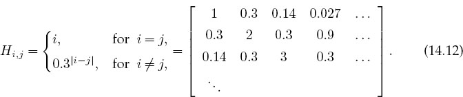
Because the Hamiltonian is almost diagonal, the eigenvalues should be close to the values of the diagonal elements and the eigenvectors should be close to N-dimensional unit vectors. For the present problem, the H matrix has dimension N χ N ![]() 2000 × 2000 = 4,000,000, which means that matrix manipulations should take enough time for you to see the effects of optimization. If your computer has a large supply of central memory, you may need to make the matrix even larger to see what happens when a matrix does not all fit into RAM.
2000 × 2000 = 4,000,000, which means that matrix manipulations should take enough time for you to see the effects of optimization. If your computer has a large supply of central memory, you may need to make the matrix even larger to see what happens when a matrix does not all fit into RAM.
We find the solution to (14.11) via a variation of the power or Davidson method. We start with an arbitrary first guess for the eigenvector c and use it to calculate the energy corresponding to this eigenvector,4
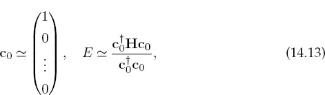
where c†0 is the row vector adjoint of c0. Because H is nearly diagonal with diagonal elements that increases as we move along the diagonal, this guess should be close to the eigenvector with the smallest eigenvalue. The heart of the algorithm is the guess that an improved eigenvector has the kth component

where k ranges over the length of the eigenvector. If repeated, this method converges to the eigenvector with the smallest eigenvalue. It will be the smallest eigenvalue since it gets the largest weight (smallest denominator) in (14.14) each time. For the present case, six places of precision in the eigenvalue are usually obtained after 11 iterations. Here are the steps to follow:
• Vary the variable err in tune that controls precision and note how it affects the number of iterations required.
• Try some variations on the initial guess for the eigenvector (14.14) and see if you can get the algorithm to converge to some of the other eigenvalues.
• Keep a table of your execution times versus technique.
• Compile and execute tune.f90 and record the run time. On Unix systems, the compiled program will be placed in the file a.out. From a Unix shell, the compilation, timing, and execution can all be done with the commands
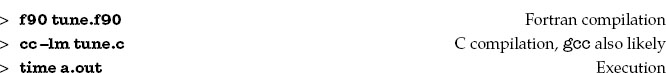
Here the compiled Fortran program is given the (default) name a.out, and the time command gives you the execution (user) time and system time in seconds to execute a.out.
• As indicated in §14.14.3, you can ask the compiler to produce a version of your program optimized for speed by including the appropriate compiler option:
> f90 –O tune.f90
Execute and time the optimized code, checking that it still gives the same answer, and note any speedup in your journal.
• Try out optimization options up to the highest levels and note the run time and accuracy obtained. Usually –O3 is pretty good, especially for as simple a program as tune with only a main method. With only one program unit we would not expect –O4 or –O5 to be an improvement over –O3. However, we do expect –O3, with its loop unrolling, to be an improvement over –O2.
• The program tune4 does some loop unrolling (we will explore that soon). To see the best we can do with Fortran, record the time for the most optimized version of tune4.f90.
• The program Tune.java in Listing 14.5 is the Java equivalent of the Fortran program tune.f90.
• To get an idea of what Tune.java does (and give you a feel for how hard life is for the poor computer), assume ldim =2 and work through one iteration of Tune by hand. Assume that the iteration loop has converged, follow the code to completion, and write down the values assigned to the variables.
• Compile and execute Tune.java. You do not have to issue the time command since we built a timer into the Java program (however, there is no harm in trying it). Check that you still get the same answer as you did with Fortran and note how much longer it takes with Java.
• Try the –O option with the Java compiler and note if the speed changes (since this just inlines methods, it should not affect our one-method program).
• You might be surprised how much slower Java is than Fortran and that the Java optimizer does not seem to do much good. To see what the actual Java byte code does, invoke the Java profiler with the command
> javap –c Tune
This should produce a file, java.prof for you to look at with an editor. Look at it and see if you agree with us that scientists have better things to do with their time than trying to understand such files!
• We now want to perform a little experiment in which we see what happens to performance as we fill up the computer’s memory. In order for this experiment to be reliable, it is best for you to not to be sharing the computer with any other users. On Unix systems, the who –a command shows you the other users (we leave it up to you to figure out how to negotiate with them).
• To get some idea of what aspect of our little program is making it so slow, compile and run Tune.java for the series of matrix sizes ldim = 10, 100, 250, 500, 750, 1025, 2500, and 3000. You may get an error message that Java is out of memory at 3000. This is because you have not turned on the use of virtual memory. In Java, the memory allocation pool for your program is called the heap and it is controlled by the –Xms and –Xmx options to the Java interpreter java:
![]()

Listing 14.5 Tune.java is meant to be numerically intensive enough to show the results of various types of optimizations. The program solves the eigenvalue problem iteratively for a nearly diagonal Hamiltonian matrix using a variation of the power method.
• Make a graph of run time versus matrix size. It should be similar to Figure 14.13, although if there is more than one user on your computer while you run, you may get erratic results. Note that as our matrix becomes larger than ~1000 × 1000 in size, the curve sharply increases in slope with execution time, in our case increasing like the third power of the dimension. Since the number of elements to compute increases as the second power of the dimension, something else is happening here. It is a good guess that the additional slowdown is due to page faults in accessing memory. In particular, accessing 2-D arrays, with their elements scattered all through memory, can be very slow.
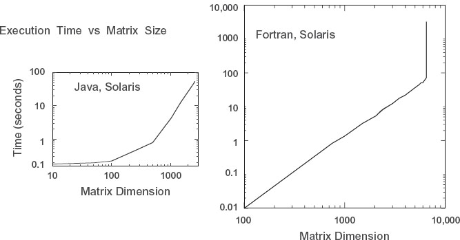
Figure 14.13 Running time versus dimension for an eigenvalue search using Tune.java and tune.f90.
• Repeat the previous experiment with tune.f90 that gauges the effect of increasing the ham matrix size, only now do it for ldim = 10, 100, 250, 500, 1025, 3000, 4000, 6000,…. You should get a graph like ours. Although our implementation of Fortran has automatic virtual memory, its use will be exceedingly slow, especially for this problem (possibly a 50-fold increase in time!). So if you submit your program and you get nothing on the screen (though you can hear the disk spin or see it flash busy), then you are probably in the virtual memory regime. If you can, let the program run for one or two iterations, kill it, and then scale your run time to the time it would have taken for a full computation.
• To test our hypothesis that the access of the elements in our 2-D array ham [i][j] is slowing down the program, we have modified Tune.java into Tune4.java in Listing 14.6.
• Look at Tune4.java and note where the nested for loop over i and j now takes step of Δi = 2 rather the unit steps in Tune.java. If things work as expected, the better memory access of Tune4.java should cut the run time nearly in half. Compile and execute Tune4.java. Record the answer in your table.
• In order to cut the number of calls to the 2-D array in half, we employed a technique know as loop unrolling in which we explicitly wrote out some of the lines of code that otherwise wouldbe executed implicitlyasthe for loop went through all the values for its counters. This is not as clear a piece of code as before, but it evidently, permits the compiler to produce a faster executable. Tocheck thatTuneandTune4actuallydothesame thing, assumeldim =4and run through one iteration of Tune4.java by hand. Hand in your manual trial.

Listing 14.6 Tune4.java does some loop unrolling by explicitly writing out two steps of a for loop (steps of 2.) This results in better memory access and faster execution.
14.15 Programming for the Data Cache (Method)
Data caches are small, very fast memory used as temporary storage between the ultrafast CPU registers and the fast main memory. They have grown in importance as high-performance computers have become more prevalent. For systems that use a data cache, this may well be the single most important programming consideration; continually referencing data that are not in the cache (cache misses) may lead to an order-of-magnitude increase in CPU time.
As indicated in Figures 14.2 and 14.14, the data cache holds a copy of some of the data in memory. The basics are the same for all caches, but the sizes are manufacturer-dependent. When the CPU tries to address a memory location, the cache manager checks to see if the data are in the cache. If they are not, the manager reads the data from memory into the cache, and then the CPU deals with the data directly in the cache. The cache manager’s view of RAM is shown in Figure 14.14.
When considering how a matrix operation uses memory, it is important to consider the stride of that operation, that is, the number of array elements that are stepped through as the operation repeats. For instance, summing the diagonal elements of a matrix to form the trace

involves a large stride because the diagonal elements are stored far apart for large N. However, the sum
![]()
has stride 1 because adjacent elements of x are involved. The basic rule in programming for a cache is
• Keep the stride low, preferably at 1, which in practice means.
• Vary the leftmost index first on Fortran arrays.
• Vary the rightmost index first on Java and C arrays.
14.15.1 Exercise 1: Cache Misses
We have said a number of times that your program will be slowed down if the data it needs are in virtual memory and not in RAM. Likewise, your program will also be slowed down if the data required by the CPU are not in the cache. For high-performance computing, you should write programs that keep as much of the data being processed as possible in the cache. To do this you should recall that Fortran matrices are stored in successive memory locations with the row index varying most rapidly (column-major order), while Java and C matrices are stored in successive memory locations with the column index varying most rapidly (row-major order). While it is difficult to isolate the effects of the cache from other elements of the computer’s architecture, you should now estimate its importance by comparing the time it takes to step through the matrix elements row by row to the time it takes to step through the matrix elements column by column.

Figure 14.14 The cache manager’s view of RAM. Each 128-B cache line is read into one of four lines in cache.
By actually running on machines available to you, check that the two simple codes in Listing 14.7 with the same number of arithmetic operations take significantly different times to run because one of them must make large jumps through memory with the memory locations addressed not yet read into the cache:

Listing 14.7 Sequential column and row references.
14.15.2 Exercise 2: Cache Flow
Test the importance of cache flow on your machine by comparing the time it takes to run the two simple programs in Listings 14.8 and 14.9. Run for increasing column size idim and compare the times for loop A versus those for loop B. A computer with very small caches may be most sensitive to stride.

Listing 14.8 GOOD f90, BAD Java/C Program; minimum, maximum stride.

Listing 14.9 BAD f90, GOOD Java/C Program; maximum, minimum stride.
Loop A steps through the matrix Vec in column order. Loop B steps through in row order. By changing the size of the columns (the rightmost Fortran index), we change the step size (stride) taken through memory. Both loops take us through all the elements of the matrix, but the stride is different. By increasing the stride in any language, we use fewer elements already present in the cache, require additional swapping and loading of the cache, and thereby slow down the whole process.
14.15.3 Exercise 3: Large-Matrix Multiplication
As you increase the dimensions of the arrays in your program, memory use increases geometrically, and at some point you should be concerned about efficient memory use. The penultimate example of memory usage is large-matrix multiplication:
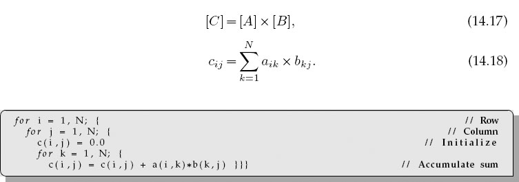
Listing 14.10 BAD f90, GOOD Java/C Program; maximum, minimum stride.
This involves all the concerns with different kinds of memory. The natural way to code (14.17) follows from the definition of matrix multiplication (14.18), that is, as a sum over a row of A times a column of B. Try out the two code in Listings 14.10 and 14.11 on your computer. In Fortran, the first code has B with stride 1, but C with stride N. This is corrected in the second code by performing the initialization in another loop. In Java and C, the problems are reversed. On one of our machines, we found a factor of 100 difference in CPU times even though the number of operations is the same!
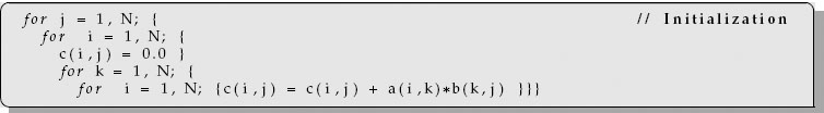
Listing 14.11 GOOD f90, BAD Java/C Program; minimum, maximum stride.
1 Some experts define our medium grain as coarse grain yet this distinction changes with time.
2 Presumably there is an analogy between the heroic exploits of the son of Ecgtheow and the nephew of Hygelac in the 1000 C.E. poem Beowulf and the adventures of us common folk assembling parallel computers from common elements that have surpassed the performance of major corporations and their proprietary, multi-million-dollar supercomputers.
3 Personal communication, Yuefan Deng.
4 Note that the codes refer to the eigenvector c0 as coef.