
2 Setting the stage
It is worthwhile to have a short look9 at the state of the art of computing at the end of World War II. Most of these computing devices were analog in nature with only a few digital computers, which were still considered being inferior to analog computers.10 Most of these developments were the direct result of military requirements like fire-control systems, the computation of firing tables etc.
The technologies available at the end of this war and the experiences gathered by engineers and scientists who devoted their knowledge to the application of automatic computing devices to all sorts of problems, would lead to an unprecedented flourishing of electronics in general and computers in particular. The ideas invented during the years of war were so fruitful that they would inspire a whole generation of engineers and scientists. Eventually, the result of their work would be the ubiquitous computing devices on which our everyday lives depend so heavily. The most important and most neglected of these computers are those machines most people never see: Control systems, ranging from small embedded computers which control simple machinery like a household appliance to heavily interconnected systems with global influence and importance. These systems take care of the consumables we need, they control the flight of our airplanes, they direct the traffic in our cities etc. Without these computers our civilization would invariably fail to exist and most of these devices owe to early developments after World War II, the most notable of those being Whirlwind and AN/FSQ-7.
2.1 Computers until 1945
Of all the various computing systems developed during World War II, most machines were so-called analog computers,11 which are based on the principle of implementing a model of a problem to be solved. Early such analog computers were purely mechanical devices like VANNEVAR BUSH’S12 differential analyzers, the first of which was completed in 1931 at the Massachusetts Institute of Technology, MIT for short. Similar mechanical devices were built by DOUGLAS RAYNER HARTREE13 and ARTHUR PORTER14 at Manchester University in 1934, by a group led by SVEIN ROSSELAND15 and many more. As powerful as these machines were, from a mathematical point of view, they were big, heavy and programming was a time consuming task. Programming back then required one to connect the various computing elements like summers, integrators, multipliers and the like with gears and rods, a task that often required hours and sometimes days to perform. This was alleviated a bit with the development of electromechanical differential analyzers. These still used mechanical computing elements but relied on intricate electrical servo-systems to interconnect the computing elements. Now the task of programming only required rewiring of a central patch-panel.
While these general-purpose analog computers were mostly one-of-a-kind machines, there was high demand for special-purpose analog computers which were employed aboard ships, submarines and on land for tasks like automatic range keeping and fire-control. 16
Already during World War II it became clear that the days of these large, heavy and intricate mechanisms which required labor-intensive maintenance on a regular schedule were numbered. Electronic analog computers were about to take over. As so often, when the time for an idea has come, electronic analog computers were developed independently in the United States of America by GEORGE ARTHUR PHILBRICK17 and in Germany by HELMUT HOELZER.18 While PHILBRICK’s machine, called Polyphemus, due to its appearance (a rack with a single oscilloscope mounted on the top while the analog computer itself occupied the lower part), was aimed at process-simulation, the machines developed by HOELZER had their roots in the war-time development of the A4.19
From the perspective of this book, HOELZER’s developments are especially interesting, since they not only produced radically novel devices which advanced the state of the art of their time but they also were the result of a war-time development. He not only developed the first truly general-purpose electronic analog computer,20 which by the way was used well after the war during the development of the Redstone and Jupiter rocket as well as for the design of the first satellite of the United States, Explorer I.21 In addition to this, he developed the so-called Mischgerät22 which was the world’s first fully electronic on-board flight computer that controlled the flight of the A4 rocket.23
Only a few digital computers were actually developed before and during World War II. One of the early pioneers of digital computers was KONRAD ZUSE24 who built the first binary, program-controlled, although not stored-program, computer, known as the Z3 which was followed by the quite successful Z4. This latter machine was not destroyed during the war as the Z3 and was used successfully for quite some years at the ETH Zürich in Switzerland.25
Another development of ZUSE during World War II were two special-purpose computers, the S1 and S2.26 These machines were intended to automatically compute corrections for wings of glide bombs like the Hs 293. One especially remarkable feature of the more sophisticated S2 was the existence of an analog-digital-converter which allowed the system to compute values based on measurements transmitted directly to the computer. Due to constraints caused by the ongoing war, all of ZUSE’s machines were based on relays as those found in telephone exchanges, although the idea of using vacuum tubes as the active elements in his computers had already received quite some thought.
Other digital computer developments were due to JOHN VINCENT ATANASOFF27 and CLIFFORD EDWARD BERRY28 who developed the ATANASOFF-BERRY Computer, ABC for short, beginning in the late 1930s. This machine was completed in 1942.29 It used a binary representation of data but was not truly programmable – in fact, the ABC was a special-purpose machine30 aimed at the solution of systems of linear equations.
A much larger scale development in the field of programmable digital computers was done under the auspices of HOWARD HATHAWAY AIKEN31 and led to the Automatic Sequence Controlled Calculator, ASCC for short.32 This system had breathtaking dimensions compared with other developments like those described above. It weighed about 4.5 tons and measured 51 feet in length, eight feet in height and two feet in depth and was entirely electromechanical.33
In 1943 JOHN WILLIAM MAUCHLY34 and JOHN ADAM PRESPER ECKERT35 began the development of ENIAC, the Electronic Numerical Integrator and Computer, shown in figure 2.1, which was originally intended to calculate artillery firing tables.36 Eventually ENIAC, which was put into operation on February 14th, 1946, turned out to be the largest fully electronic digital computer in its day, containing about 18,000 vacuum tubes, 1,500 relays, 7,200 semiconductor diodes and tens of thousands of capacitors and resistors. The overall machine weighed about 27 tons and consumed 140 kW.37 Although naysayers doubted that a machine using so many vacuum tubes could perform any useful work at all between the presumably short periods between two failures, ENIAC proved them wrong.38 The basis for this success was a conservative circuit design in conjunction with some simple operating procedures like not turning the computer on and off but let it run to reduce thermal stress on the tubes.

Figure 2.1: U.S. Army photo of ENIAC (initial installation at the Moore School of Electrical Engineering, it was transferred to the Ballistic Research Laboratories, Aberdeen Proving Ground, in 1947), cpl. IRWIN GOLDSTEIN in the foreground sets switches on one of ENIAC’s function tables.39
Although ENIAC came too late to calculate firing tables for artillery shells it was put into use for a variety of mainly military projects, the first of which was suggested as early as 1945 by JOHN VON NEUMANN:40
“In early 1945, as the construction of the ENIAC was nearing completion, VON NEUMANN raised the question with [physicist STANLEY] FRANKEL and METROPOLIS of using it to perform the very complex calculations involved in hydrogen bomb design. The response was immediate and enthusiastic. Arrangements were made by VON NEUMANN on the basis that the ’Los Alamos problem’ would provide a much more severe challenge to the ENIAC on its shakedown trial.”41
These calculations proved to be quite successful which in 1946 led the director of Los Alamos to write a letter to the Moore School stating that “the complexity of these problems is so great that it would have been impossible to arrive at any solution without the aid of ENIAC.”42 In fact, ENIAC proved to be such a valuable tool that the press was enthusiastic and created terms like “giant brain” and others. A typical report from the ENIAC unveiling read like this:
“Mathematical brain enlarges man’s horizons. . . A new epoch in the history of human thought began last night. The scope and area in which man’s brain can grasp, predic[t], control suddenly opened outward into the distance with revelation of section construction during the war of a 30 ton mathematical brain that solves the unsolvable.”43
Other headlines were equally enthusiastic and exaggerating. The time-honored London Times featured an article about ENIAC with the headline “An Electronic Brain: Solving Abstruse Problems; Valves with a Memory” – too much anthropomorphism for DOUGLAS RAYNER HARTREE,44 a renowned British mathematician and physicist. He sent a sharply-worded letter to the editor but to no avail. The notion of the giant or electronic brain persisted.45
It turned out that ENIAC’s architecture, which had few things in common with today’s computer architectures and more closely resembled a so-called Digital Differential Analyzer,46 a digital variant of an analog computer, was not suitable for future developments, but more importantly, this machine proved that computers involving tens of thousands of delicate vacuum tubes were not the maintenance nightmare that had been predicted. Although not comparable with today’s machines in terms of reliability and mean time to repair, MTTR for short, it was reliable enough to allow the solution of problems which were next to unthinkable before. In this respect ENIAC deserves highest respect for encouraging not only scientists and engineers to employ highly complex electronic computers but also for being the archetypal giant brain that would shape the picture of a computer for the following years.
2.2 Basics of vacuum tube circuits
Since many of today’s readers may not be familiar with vacuum tube circuits any more, a short digression might be allowed since Whirlwind and AN/FSQ-7 both were vacuum tube digital computers. Some basic knowledge about vacuum tubes, these nearly forgotten active circuit elements, is helpful for the following chapters.
Although there was a plethora of vacuum tubes in use until the late 1960s when transistors finally won the battle as the all-purpose active element, we will focus only on diodes and triodes to get an impression of how basic vacuum tube circuits work.47 Basically the simplest vacuum tube, the diode consists of a heated cathode which emits electrons and an anode which collects those electrons.
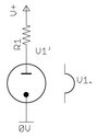
Figure 2.2: Basic vacuum diode circuit
Figure 2.2 shows the schematic of a simple circuit employing a vacuum diode V1. The cathode is typically made from nickel and is coated with an alkaline earth metal oxide which gives off electrons rather easily. It is depicted by the dot connected to circuit ground while the anode, which is also often called plate, is represented by the plate-like symbol connected to the resistor R1. The symbol to the right of the tube itself denotes the heater which heats the cathode to 800–1000° C. Such an arrangement is called an indirectly heated cathode – simpler tubes use the emission from the glowing heater itself and are called directly heated. Indirectly heated vacuum tubes have some advantages, especially the fact that heater and cathode are essentially isolated against each other. The heater won’t be shown in following schematics.
If the anode is at a positive potential with regard to the cathode, as shown in figure 2.2, electrons will flow from cathode to anode and the tube is said to be conducting, i. e. a current flows through the resistor R1.48 If the anode is negative with respect to the cathode, its potential will repel the electrons and no current flows. Thus a vacuum diode allows current to flow in one direction only – quite like a modern semiconductor diode.49
A far more interesting device is the triode which is based on a vacuum diode which has been extended by a so-called control grid which normally is just a fine wire mesh placed between the electron emitting cathode and the anode. If this grid is left unconnected, the tube just behaves like a vacuum diode, but applying a more or less negative voltage to this grid allows for modulation of the electron flow from the cathode to the anode, hence the name control grid. The interesting thing about this means of control is that a triode is controlled by a voltage, not a current as would be the case in a bipolar transistor. Thus a vacuum triode may be compared to a depletion field-effect transistor.
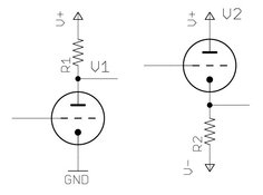
Figure 2.4: Basic vacuum triode circuits, inverter left and cathode follower right

Figure 2.5: Inverter with output network
Figure 2.3 shows a typical so-called twin-triode of the 1940s, i. e. two triodes sharing a common evacuated glass envelope. In the middle of the front triode the fine mesh comprising the grid can be seen, surrounding the thin and long indirectly heated cathode which in turn contains the heater windings. The grid in turn is surrounded by two halves of the anode. Two such triodes are housed next to each other. At the bottom the wires connecting heaters, cathodes, grids and anodes to the socket connectors protrude through the glass envelope.
Figure 2.4 shows two basic triode circuits. In both cases, the triode and a resistor form a controlled voltage divider. The circuit on the left is a so-called inverter: If the grid is at ground potential or slightly above,50 current flows from cathode to anode, so the junction between the plate resistor R1 and the plate will be pulled to ground potential. Since the tube and the resistor form a voltage divider, the output potential at the plate-resistor junction will be rather low with respect to ground. If the grid voltage is made negative with respect to the cathode, the flow of electrons will be blocked to a certain degree which depends on the grid and plate voltage and the tube’s overall characteristics.
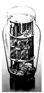
Figure 2.3: Cutaway view of a twin-triode 6AS7G (see [BARRY 1949][p. 551])
So a negative voltage at the control grid causes the output of this left circuit to be positive while a zero or slightly positive grid voltage will cause the output to go low which makes this circuit behave like an inverter. If the control grid were connected to a number of different signal sources, each decoupled by a semiconductor diode, a basic digital gate like a NAND, short for Not And, will result.
The circuit shown on the right in figure 2.4 is a so-called cathode follower. Here the resistor and the tube have switched places, so that a conducting tube (non-negative control grid voltage) will cause a positive output while a negative grid voltage will cause a negative output. So, basically, the cathode follower is a non-inverting circuit and can be used readily to amplify a digital signal.
In practice these two circuits are much too simplified for use in high-speed computer circuits. One of the main problems are stray capacitances in the tube itself and its wiring especially with respect to the output lines. Controlling the grid of either the inverter or the cathode follower with a square wave signal will realistically result in an output signal which deviates more or less from a square wave, since the rising and falling edges will be deformed according to an exponential curve due to those stray capacitances. The basic solution to this problem is shown in figure 2.5 which resembles an inverter with the addition of an output network consisting of two resistors R2 and R3 in series where one resistor, R2, is paralleled by a capacitor C1. When the polarity of the output signal changes, a rather large current flows through C1 thereby counteracting the deformation of the rising or falling edges caused by the unavoidable stray capacitances. Given the large physical dimensions of vacuum tube based computers where signal lines often have a length in meters rather than centimeters, these capacitances of the output lines would make high-speed operation impossible without such countermeasures.
Figure 2.6 shows one of the most fundamental digital circuits of all, a flip-flop. This is a bistable circuit which can be used to store one bit or to build counters etc. It basically consists of two inverters connected in a crosswise fashion: If the left tube conducts, the potential at its anode which is connected to the control grid of the right triode via R3, is at a negative potential through R6 so the right tube does not conduct. Applying a positive impulse to the grid of the right tube then lets this tube conduct, which in turn blocks the left triode which will then hold the right tube in the conducting state.
Figure 2.7 shows a typical early application of such a triode flip-flop: A ring-counter circuit from ENIAC. In contrast to today’s computers, ENIAC was a decimal instead of a binary machine. As if this number representation was not unusual enough, ENIAC used such ring-counters consisting of ten stages to represent a single decimal digit, so a single accumulator51 capable of storing one ten-digit number consisted of ten such flip-flops, each requiring two triodes or one twin-triode.52
This ring-counter consists of ten flip-flop stages similar to that shown in figure 2.6. Each stage is coupled crosswise between the grids and anodes by means of an RC-combination53 and is in one of two stable states at each time. These ten flip-flop stages are in turn coupled by capacitors connecting the anode of the right triode of a pair with the control grid of the right anode of the flip-flop right next to it.

Figure 2.6: Basic flip-flop circuit with two triodes
The shading denotes the active triodes – the leftmost flip-flop is in the set state while the remaining nine flip-flops are all reset. It is interesting to note how this circuit is set to a particular value: Its input is shown on the right – incoming negative pulses are applied to the cathodes of the left triodes of each flip-flop element. A negative pulse will only reset the one particular flip-flop which was in the set state. This reset-operation results in a pulse transmitted through the interstage coupling capacitor to the next flip-flop in the chain which will in turn be set.
It is clear that such a number-representation requires much more circuit elements per digit than even a decimal based binary representation like the so-called BCD-code.54 This representation uses ten out of the 16 possible states of four bits. So storing a single BCD digit would have required only four flip-flops with some additional circuitry to avoid illegal states not representing a decimal digit. Nevertheless the savings would have been substantial. Even more savings would have been possible if a pure binary representation of values in the computer had been chosen from the beginning.
Due to habit and fear of radical changes like switching to a then uncommon number system, many early computers relied on the decimal number system yielding unnecessarily complex circuits as seen from today’s perspective. It is interesting to note that KONRAD ZUSE not only decided to use a pure binary representation of values at the very beginning of his developments in the 1930s55 but also incorporated special circuits in his machines which performed the necessary conversions between the external decimal and the internal binary number representation.

Figure 2.7: Typical ring-counter circuit as used in ENIAC (see [STIFLER et al. 1950][p. 24])
2.3 Toward Whirlwind and beyond
Only military applications could offer the necessary amount of financial backing and staffing necessary to build a large scale stored-program digital computer back in the early days of computing. One particularly important and complex problem of World War II was the simulation of aircraft for research as well as for training purposes. Training new pilots in real aircraft not only bound many aircraft in the training centers instead of using them in battle, but was also a dangerous way to teach the art of flying. Not too surprisingly, many casualties among the pilots and even more damaged aircraft were the result, rendering the traditional way of training more than ineffective under the immense pressure of an ongoing war.
Intrigued by the problem of aircraft simulation,56 LUIS DE FLOREZ57 – characterized as being a “brilliant [and] flamboyant engineer”58 – asked his alma mater, the MIT, to build a flight simulator. This machine should be used for research purposes as well as for training naval bomber flight crews without exposing them to the unnecessary risks of real flights. This request should finally lead to the development of Whirlwind,59 sponsored by the Office of Naval Research (ONR), which should not only become the icon of an era but extend the frontiers of electronic computing in an unprecedented way, being the first real-time digital computer.
When work on the proposed flight simulator began, it was decided to build an analog computer according to the then state of the art in electronic circuit design. This seemed a plausible decision since flight simulation was and still is one of the archetypal problems requiring real-time computation, something that was thought to be possible only by analog computing. Instead of building a training device, it was decided in about 1944 to focus on research on the stability and control characteristics of large aircraft in general by building an analog computer, the Aircraft Stability and Control Analyzer (ASCA).
As early as in 1946, JAY WRIGHT FORRESTER60 decided to abandon the analog computer approach to ASCA and start development of a novel stored-program digital computer,61 which eventually would become the world’s first real-time computer suitable for control and simulation tasks. As a direct result of this shift of focus, the work previously done at the Servomechanisms Laboratory62 was relocated to a new laboratory, the Digital Computer Laboratory (DCL), which was set up to take over the task of developing this new digital computer.63 The DCL then operated as a division of the Servomechanisms Laboratory until it became an independent laboratory for digital computers and their applications.64
Let us digress a bit and have a look at the situation of air defense right after the end of World War II: Back then the United States operated more than 70 so-called Ground Control Intercept (GCI) sites which were rather intricate installations, each consisting of one or two search radars, height-finder radars, and various ground-to-air and air-to-ground communication facilities to direct intercept aircraft to approaching bombers and the like.65
First contacts between the Air Defense Evaluation Group (ADSEC) and the team working on Whirlwind were made as early as 1947.66 When the Soviet Union successfully detonated their first nuclear weapon in 1949, it became clear that the United States were no longer the only global power armed with nuclear weapons and some action would be necessary to assure that a first-strike by the Soviet Union could be answered immediately to assure a climate of mutual deterrence. Thus in November 1949 GEORGE EDWARD VALLEY Jr.67 from MIT proposed to THEODOR VON KÁRMÁN68 that a general study of air defense requirements should be undertaken immediately to be prepared for any possible Soviet aggression.69
The results of this study turned out to be devastating. In 1950 the ADSEC under GEORGE E. VALLEY and the Weapon Systems Evaluation Group (WSEG) reported that the current air defense system of the United States, more or less a remnant of the systems in operation at the end of World War II, was no longer sufficient for current and future threats involving nuclear weapons and strategic long-range bombers capable of delivering such weapons. Rather drastically, the Scientific Advisory Board (SAB) remarked that the current manual system was in fact “lame, purblind, and idiot-like” with extra emphasis on the last point:
“[Of] these comparatives, idiotic is the strongest. It makes little sense for us to strengthen the muscles if there is no brain; and given a brain, it needs good eyesight.”70
It was clear that future requirements for such an air defense system would be substantially different from those encountered and mastered quite well by means of manual systems during World War II:
“The earth’s curvature meant that hundreds, if not thousands, of radars would be required to detect low-flying aircraft... There was no conceivable way in which human radar operators could be employed to make [the necessary] calculations for hundreds of aircraft as detected from such a large number of radars, nor could the data be coordinated into a single map if the operators used voice communications. The [. . . ] computations were straightforward enough. [. . . ] It was doing all that work in real time that was impossible.”71
These findings led to a study of the overall task of air defense which was performed as Project Charles at the MIT. This project suggested that the existing manual system should be upgraded to fill the most pressing immediate needs while in parallel a laboratory which would become known as the Lincoln Laboratory72 should be established to work on a so-called transition system which would eventually lead to the development of the AN/FSQ-7 and SAGE.
It is interesting to note that FORRESTER and some of his colleagues already proposed the application of a computer to the overall air defense task two years earlier, back in 1948, which pretty much antedates the findings of the ADSEC and WSEG and their conclusions:
“An example of a requirement in the solution of tactical problems is found in the interception of supersonic missiles. Here there is need for [a] combined computer and control system which can:
- Automatically receive radar and other information from multiple locations,
- Correlate this with past information,
- Distinguish between types of missiles and distinguish missiles from aircraft based on identifying information and trajectories,
- Predict trajectories to the impact point (if flight is uncontrolled),
- Assess possible damage and importance of defense action to permit concentration of defense against the most dangerous missiles,
- Take rapid automatic defensive action in selecting launching location and firing defensive missiles, where time is too short for human intervention,
- Carry on these operations with a minimum of equipment,
- Possess the required flexibility to avoid the need for redesigning to meet changing tactical situations and the appearance of new weapons of either offense or defense.”73
In January 1950 paths crossed, when GEORGE E. VALLEY learned from JEROME BERT WIESNER74 – whom he met by chance in a hall of MIT – that there already was a computer named Whirlwind that was “sitting up for grabs on the MIT campus”.75 This should be the beginning of one of the biggest adventures in digital computing and would finally lead to the development of the first large scale nationwide computer network for the purpose of air defense. At this time Whirlwind76 was already operating partially while development of and on the machine was still ongoing.77 Whirlwind was completed in stages with the overall system being fully operational in 1951.78
Already in 1950, an experimental system based on Whirlwind as its central component was set up to demonstrate the feasibility of the application of a large scale digital computer to the air defense problem.79 Since Whirlwind was still in an early stage of development, only 256 memory cells of electrostatic memory and an additional 32 memory locations of so-called test memory were available.80 Accordingly, the overall program to perform the track-while-scan operation with all necessary constants etc. had to fit into this tiny amount of memory, next to incredible from today’s point of view.81
“The objective of the first air defense experiments and studies was the use of the Whirlwind Computer to perform the necessary computational and data-processing functions associated with:
- automatic track-while-scan (Track While Scan (TWS)); that is, the automatic tracking and display of selected aircraft using data obtained from a continuously-rotating search radar, and
- the automatic track-while-scan of selected aircraft and the computation of the heading instructions necessary to guide one aircraft – the interceptor – on a collision course with a second aircraft – the target. These interception computations were to be such that they could be used for the mid-course phase of the interception, leading to a closing phase under the direction of airborne intercept (Airborne Intercept (AI)) radar.”82
To accomplish this task, Whirlwind –located at the MIT in Boston – was coupled to a Microwave Early Warning (MEW) radar set at Bedford airport, about 12 miles away from Boston. To transmit the radar data to Whirlwind, an already existing prototype Digital Radar Relay (DRR) was used.83 The other communications link to the interceptor aircraft was implemented by means of a traditional voice radio link.
First experiments during the fall of 1950 were not successful due to problems with the DRR but in the spring of 1951 actual tests involving aircraft supplied by the Instrumentation Laboratory of the MIT and the Air Force Cambridge Research Center (AFCRC) commenced. These tests were highly successful as [ISRAEL 1951][p. 6] notes:84
“These tests established that the computer with a storage capacity of 256 registers85 could successfully track five aircraft86 or could track two aircraft, guiding one on a collision course interception with the other. About ten interception flight tests were attempted and completed through June of 1951; the final separations of the target and the interceptor aircraft as their paths crossed averaged between 500 and 1500 yards.”
Due to the restrictions of the MEW radar system, the analog-to-digital conversion equipment,87 the DRR, and Whirlwind, some simplifications were necessary to perform these tests: First of all only two dimensions were taken into account, so target and interceptor were assumed to be acting in the same horizontal plane. Azimuth data was converted into an eight bit value, so an angular resolution of about 1.4° could be achieved. Range data was converted into a seven bit value so values up to 127 miles could be represented. This range information was padded with a 0 bit yielding an eight bit byte, too. For data transmission the azimuth byte was padded with two bits 01 while the range data was padded with 00. Transmission of one such ten bit word took 1/ 50 of a second.
On the receiving end these ten bits were stored in a 16 bit wide so-called Flip-Flop Register which could be addressed as a normal memory location.88 Writing into this register was synchronized with the operation of the computer to ensure data integrity by blocking write accesses while the computer reads this particular register. Since Whirlwind did not feature interrupts, a polling scheme was employed which checked this register more frequent than every 1/ 50th of a second for new data.89
During these studies it became clear that multiplication operations were executed much more often than divisions which was due to the fact that the data transmitted by the radar system via the DRR naturally represented polar coordinates while all computations took place in Cartesian coordinates due to the Cartesian nature of the display system, so a lot of coordinate transformations had to be performed. This observation would have a great impact on the design of the arithmetic unit of the later AN/FSQ-7 since an implicit shift was built into its addition operation to speed up multiplications. The detrimental effect this had on divisions was accepted and programmers tried to avoid divisions when- and wherever possible.
Nearly all of the experiments based on the Bedford radar station used so-called manual acquisition in which a human operator had to select a particular target aircraft to be tracked. This acquisition process was implemented by a light gun, which mainly consisted of a photomultiplier tube built into a gun-like enclosure so that an operator could point the tube’s window to a particular area of interest on the display screen. When the object displayed in that area of the display was updated the next time by the computer, an impulse was generated by the light gun’s circuitry which reset a bit in a Flip-Flop register. The computer then had to check this particular bit after drawing every single object to determine which object the light gun was pointed to when its trigger was pulled.
These early experiments also led to the development of the radar mapper: These devices were used to remove clutter which was especially pronounced at near distances. A Plan Position Indicator (PPI) display showed incoming radar data; above this display, a photomultiplier tube with the necessary optics was mounted so that it could “see” the overall display. This tube registered only the blue flash of light which was emitted when the display was updated. To remove clutter, those areas of the display tube where static features like land marks etc. were displayed, could be covered by an opaque mask which was painted manually onto the display tube’s surface. Thus the photomultiplier assembly only generated an output signal when an update on an area of the PPI was performed which was not masked. This signal was then used to gate data transmission to the receiving computer, effectively suppressing any clutter signals.90
| Register length | 16 binary digits, parallel |
| Speed | 20,000 single-address operations per second |
| Storage capacity | Originally 256 registers |
| Recently 320 registers | |
| Presently 1,280 registers | |
| Target 2,048 registers | |
| Order type | Single-address, one order per word |
| Numbers | Fixed point |
| Basic pulse repetition frequency | 1 megacycle |
| 2 megacycles (arithmetic element only) | |
| Tube count | 5,000, mostly single pentodes |
| Crystal count | 11,000 |
Table 2.1: Characteristics of Whirlwind as of 1951 (see [EVERETT 1951][p. 71])
To get an impression of the amount of computing power available at the time of these early experiments, table 2.1 shows the characteristics of Whirlwind as of 1951. Apart from the scarce amount of memory available, another aspect is remarkable: That of the rather short word length. Other contemporary machines, which were mainly aimed at scientific and engineering computations, featured word lengths of 36 or 40 bits while Whirlwind only used a 16 bit machine word. The rationale behind this decision was that it was preferable and easy to trade machine time for precision by using subroutines to perform multi-precision computations instead of building a much larger system involving much more delicate components like vacuum tubes that were error prone and would not only complicate the computer unnecessarily but turn the machine into a maintenance nightmare. FORRESTER remembers:
“Making the decision to build Whirlwind [. . . ] with a 16 binary digit register length was tremendously hard for us. The mathematicians were up in arms. They thought it was too short to be of any possible use. We defended it at that time on the basis that it was a demonstration of feasibility and we would build a 32 or a 36 bit computer when the right time came. [. . . ] Selecting 16 bits was not a useless register length for computing, only a serious short term political problem.”91
| STORAGE (16-digit words) | ||
| Magnetic-Core Storage (Magnetic-Core Storage (MS)): | ||
| 2 banks, each having 1,024 cores per digital plane; access time, 10 µs | ||
| Auxiliary Drum Storage: | ||
| 12 groups each of 2,048 registers on magnetic drum; single word or block transfer to and from MS; average access time to single word or block: 8.5 msec within a group, 16 msec to select new group; block transfer rate, 64 µs/word. | ||
| Test Storage: | ||
| 32 toggle-switch registers; 5 flip-flop register (interchangeable with any 5 toggle-switch registers). | ||
| SPEED (in microseconds) | ||
| Addition: | ||
| To get one number from MS, add it to one in Arithmetic Element (AE) | 35 | |
| To get two numbers from MS, add them, and transfer answer to MS | 100 | |
| Multiplication and Roundoff: | ||
| To get one number from MS, multiply it by one already in AE | 50 | |
| To get two numbers from MS, multiply them, transfer product to MS | 120 | |
| TERMINAL EQUIPMENT | ||
| Punched Paper Tape and Typewriters: | ||
| Flexowriter 7-hole tape (6 information, 1 index); 6-binary-digit code for letters and decimal numbers. Input to computer: mechanical tape reader (106 ms/line, 318 msec(word), photoelectric tape reader (7 msec/line, 21 msec/word); output: type punch (93 msec(line, 279 msec/word), printers (about 135 msec/character, up to 900 msec for carriage return). | ||
| Magnetic Tape: | ||
| Parallel-serial storage of binary digits in 3 pairs of nonadjacent channels (2 information pairs, 1 index pair). Redundant recording in pairs minimizes tapeflaw errors. Maximum density, 100 lines (200 binary information digits) per inch; speed, 30 inches per sec. Coded tape recording of computations enables printer to operate independently of computer. | ||
| Oscilloscope Display: | ||
| Five modified Dumont 5-inch oscilloscopes and several 16-inch magnetically deflected CRTs are available for display. X and Y axes each have 2,048 discrete positions (about 350 µs for point or vector set up and display, about 480 µs for character set up and display). Fairchild camera, automatically controlled by computer, can be used with either type. | ||
| Buffer Drum: | ||
| Magnetic drum acts as temporary storage of input and output data arriving at computer in random and asynchronous manner from multiple sources and leaving for various output devices. | ||
Table 2.2: Characteristics of Whirlwind as of 1954 (see [MANN et al. 1954][p. 1-2])
Only three years later, in 1954, Whirlwind had been expanded with a plethora of peripheral devices and the error-prone electrostatic memory (more about that later) had been replaced by the newly invented core memory – the laboratory oddity had finally evolved into a stable computer system that could be used for research and was no longer the focus of research itself. Table 2.2 shows the setup of Whirlwind in 1954 when it had reached a rather stable state. The following chapter will now describe Whirlwind and its various subsystems in more detail.